Instructions and Notes
Suggested Citation
SCIPP, 2024: Simple Planning Tool for Climate Hazards, v 2.0. Southern Climate Impacts Planning Program, https://www.southernclimate.org/resources/tools/simple-planning-tool.
About the Simple Planning Tool
This tool is a compilation of relatively easy-to-use online interactive tools, maps, and graphs to assist planners and emergency managers in Louisiana who are assessing their long-term climate risks, both historically and in the future. It is primarily designed for decision- makers who serve small- to medium-sized communities but may also be of interest to those who serve larger areas. This tool was developed with input from local and state emergency managers and planners. While it may not answer every question about a hazard’s climatology and future trend, it aims to cut through the internet clutter and point to relatively simple data tools that can be used during planning processes and in plans. The Simple Planning Tool for Climate Hazards was produced by the Southern Climate Impacts Planning Program (SCIPP, www.southernclimate.org).
In many cases, there are more tools that may assist you with developing hazards profiles. The SCIPP team throughly reviews all tools and resources included in the SPT and selects those that are most useful to a range of applications. However, you may find tools that better suit your particular needs. If you are considering using a tool that is not included in the SPT and would like the SCIPP team to review it for you, please contact us. You may also provide tool suggestions through our Feedback Form.
For tool assistance or questions, please contact scipp@southernclimate.org
About SCIPP
The Southern Climate Impacts Planning Program (SCIPP) is one of several National Oceanic and Atmospheric Administration (NOAA) Climate Adaptation Partnership (CAP) teams, formerly Regional Integrated Sciences and Assessments (RISA). SCIPP is a climate hazards and research program for the south central United States and focuses on increasing the region’s resiliency and level of preparedness for weather extremes now and in the future. The area SCIPP serves includes the 4-state region of Oklahoma, Texas, Arkansas, and Louisiana.
User Instructions
This tool is organized with expandable sections as you scroll through the webpage, and each section is displayed and accessible on the left-hand floating menu.
Hazards in this tool are alphabetically organized by climate hazard and three other hazards. As you scroll down the page, an expandable menu item is included for each hazard and describes the data limitations, definition and description, historical data tools, and climate change trends and tools. The left-hand menu also includes an expandable Hazards section that you can select a hazard from. See the list of components below to learn how each hazard section is organized.
Hazard Section Components
Data Limitations: In the dark gray box, known data limitations for the hazard are described. Knowing limitations can help one interpret data results more accurately.
Definition & Description: This section provides the definition and description of the hazard, which is required in a hazard mitigation plan. Click the blue “Copy Text” button on the top right of this section to easily copy all of the text with one click and paste it right into your plan. References for all in-text citations are located in the Acknowledgements & References section on the left-hand menu.
Historical Data: The Historical Data section shows several tools that provide freely available historical data relevant to each hazard.
- Tool Info: For each individual tool, we provide its name, period of record of the data used (some tools use multiple periods), and the source.
- Tool Description: Under the tool info, we also provide information that can be obtained from the tool and instructions on how it can be used.
- Tool Thumbnail & Link: To the right of the tool info is a thumbnail with an example image of the tool’s final product (i.e., map, graph, table). Click the blue “View the Tool” button to access the tool. (Note: In the event of a URL change, search the web using the accompanying information.)
Climate Change Trends: This section shows tools that include climate projections and future trends of the hazard (if available). It also includes a concise summary of the state-of-the-science on whether the hazard is projected to be influenced by climate change, and if so, how. Any tools in this section are organized the same as the Historical Data section.
A Note About Climate Data Availability
Data availability differs among weather variables. Some variables are easier and less costly to observe than others. For example, temperature and liquid precipitation have longer and more complete periods of record than tornadoes and freezing rain. In addition, it is not scientifically appropriate to analyze long-term trends for some hazards due to reporting differences over time. For example, the long-term trends of tornadoes, severe wind, and hail reports are biased due to population increases and advances in the ability to detect and communicate information. Refer to the data limitations portion of each hazard section for more details.
Ideally, every city or parish in Louisiana would have detailed, long-term climate records. However, even though modern science and technology have greatly advanced data collection, there are limitations that are noted above. Data products such as tables, graphs, and maps are commonly produced from single point observations, analyses that interpolate between data points (for those locations that do not have individual records), or by averaging (such as across climate divisions). Users should be aware that this document references tools that show observational points, some that show interpolation analyses, and some that show averages.
Although individual stations are often favored as they provide local data, it might not be the best choice to use a single station’s data for long-term risk analysis if it is of poor quality (i.e., has data gaps or has not been calibrated) or has a short period of record. For example, some stations have long-term temperature records that begin in the eighteenth century. Other stations, such as those operated by the Louisiana State University AgCenter, for example, have only existed since late 2001 and have a very limited number of stations. Depending on user needs, it may be more appropriate to look at data from a station that is relatively close to the desired location (i.e., not in the exact city or parish) if it has a longer period of record. In other words, if a user is looking to assess a location’s long- term risk, a nearby station with 60 or 100 years’ worth of data may be more valuable than a local station that only contains 15 years of data or has long periods of missing data. Furthermore, if a nearby station does not have a long-term record, it may be more valuable to focus on the tools with interpolated analyses or averages. These tools are acknowledged by atmospheric science professionals, including climatologists, to represent accurate and relevant data when locations are under-represented.
Using point data may also miss important events that pose a risk to the city. For example, if a strong tornado passed close to a city, using only historical tracks from within city limits would not include the event and therefore underestimate risk. Therefore, it is wise to consider nearby areas along with the particular location of interest when assessing hazard risk.
For more information on data limitations or questions regarding suspect data, contact the Louisiana State Climatologist, Dr. Barry Keim, at keim@lsu.edu or 225-578-6170.
A Note About Climate Change
The future trend portion accompanying each hazard section in this document provides concise summaries of the most up-to-date scientific knowledge regarding how climate change is or is expected to impact each hazard. The science is clear that our global climate is changing at a rate that we have not observed before in modern times, and humans are a primary influence behind this rate of change. However, the changes we are experiencing and expect to experience in Louisiana are nuanced. In many cases, only descriptive information about likely changes can be given, as climate models are currently not capable of providing skillful magnitudes of the changes. For example, models may be able to examine changes in environmental conditions favorable to storms but lack the resolution to determine likely storm severity. For climate change information that is more in-depth than that which accompanies each hazard section in this tool, please visit the resources listed in Climate Change Science and Projection Resources (under Instructions and Notes).
A Note About Impact Data
Understanding the detailed impacts of weather and climate on cities, parishes, and tribes is an important and necessary step to reduce risks and costs. Impacts of events are dependent upon characteristics of the location such as low-lying areas susceptible to flooding, soil types, housing construction, and resources available to respond and rebuild. Given disparate data sources, however, gathering comprehensive impact data and including it in the Simple Planning Tool was not possible due to resource constraints. If future resources support further research, additional versions of the Simple Planning Tool for Climate Hazards may include impact data.
Coastal Erosion
Data Limitations
Coastal erosion is complex because of the many factors that affect the changing coastline, including sea level rise, coastal flooding, subsidence, winds, and wave action. Therefore, measuring changes from erosion can be difficult. Coastal gauges are also sparse, so there is limited historical data at many locations. Satellites have greatly improved observations of eroding coasts but do not yet provide a long-term record. Long-term changes are found through archived aerial images, surveys, coastal gauge data, and satellite observations.
Definition and Description
The process by which local sea level rise, strong wave action, and coastal flooding wear down or carry away rocks, soils, and/or sands along the coast (U.S. Fed. Gov., 2021).
Coastal erosion naturally occurs through storms, strong waves, and high tides, and sea level rise exacerbates this issue. Coastal change, including from erosion and sea level rise, is measured by remote sensing (e.g., aerial photography, satellite imagery, photogrammetry, and lidar), surveys, and coastal gauge data.
Coastal erosion causes coastal property loss (infrastructure and land/beaches), reduction of wetlands/marshes, and negative impacts to the economy (e.g., transportation infrastructure, business and tourism disruption, decreased property values). Subsidence is another contributor to land loss in Louisiana. The loss of wetlands causes further impacts from tropical storms because wetlands act as a buffer to storm surge and tropical storm winds.
Louisiana accounts for 80% of coastal wetland loss in the U.S. due to coastal erosion, subsidence, and other factors. Louisiana has over 3 million acres of wetlands, and coastal erosion has caused over 35 miles of wetlands to be lost each year (LA Sea Grant 2024). Additionally, 1,900 square miles of the Louisiana coast have been lost since 1932, which accounts for about 25% of the land area since 1932 (Couvillion et al. 2017). Louisiana could experience $15-25 billion in annual damages and 14,000-22,000 annual structural damages by 2050 if no action is taken to combat land loss (CPRA 2023).
Historical Data
Coastal Change Hazards Portal
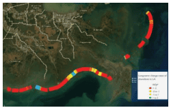
(Historical: ~150 years; short-term change: ~30 years, long-term change: ~78+ years) U.S. Geological SurveyAccess this tool to view shoreline changes due to hurricanes, coastal erosion, and sea level rise using maps of long-term historical data and projections of changes from sea level rise.
1. To view coastal erosion changes, zoom into the area of interest 2. Select Shoreline Change from the righthand menu. 3. Choose to view long-term or short-term shoreline change rates or historical shoreline positions. 4. Click Gulf of Mexico shorelines, then choose Louisiana. The map will show your selection along the Louisiana coast.
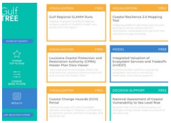
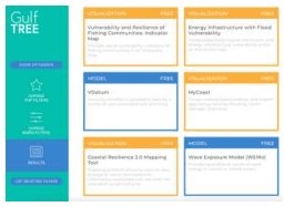
Gulf Tree
(Period of record varies by product) Northern Gulf of Mexico Sentinel Site Cooperative, Gulf of Mexico Climate Resilience Community of Practice, & Gulf of Mexico Alliance Resilience TeamThis decision support site guides users to the coastal erosion tools and resources they need along the Gulf Coast through several filters of information, including how much time and effort they’re willing to spend on the tool.
1. Choose a Filtered Search to look through all filter categories on one page or choose Guide My Search to walk through questions step by step to achieve what you’re looking for. 2a. If you chose the Filtered Search, first navigate to Geographic Scope. Click the Louisiana drop-down menu and choose Shoreline to select all coastal parishes or choose specific one(s). 2b. Under Tool Function, select what you’d like to use coastal erosion information for. 2c. Under Cost, choose Free. 2d. Under Level of Effort, choose from high, moderate, or low (will determine how advanced the tool is). 2e. Under Climate Change Themes, check the box for Sea Level Rise. 2f. Under Climate Change Topics, select the drop-down for Coastal Processes, then check the box for Erosion. 2g. Click View Tool Matches on the top right to go to the results page. Click any of the tools or resources to go to that site.
3a. If you chose Guide My Search, Gulf Tree will walk you through the same filters by asking 6 questions. For step 1 (Tool Function), check the box for why you need a coastal erosion tool, then click Submit. If you’re not sure which option to use, you can Skip this step. 3b. Step 2 (Topic Area) includes a filter for what aspect of the topic you’re interested in. Click the drop-down menu for Coastal Processes and check the box for Erosion, then click Submit. 3c. On Step 3 (Location), click the Louisiana dropdown menu, then choose Shoreline to select all coastal parishes or choose specific one(s). Then, click Submit. 3d. For Step 4 (Level of Effort), choose how much effort you’d like to put into the tool, which will determine how advanced the tool is. Then, click Submit. 3e. For Step 5 (Tool Cost), choose Free, then click Submit. 3f. Click Leave Guided Search and View Matches to go to the results page or go back to a previous page on the left menu to change your selected options. Click any of the tools or resources to go to that site. 6. To create a new search, click Reset All Filters at the top right of the results page.
Climate Change Trends
In the last 80 years, the average erosional rate of shoreline change in Louisiana was 25 ft/yr, with some areas in southeast Louisiana experiencing much higher rates of erosion coupled with high subsidence (Himmelstoss et al. 2017). The highest erosion rates in the Gulf of Mexico have occurred in Louisiana (Himmelstoss et al. 2017). Sea level rise and the potential for increased hurricane intensity increases coastal erosion, so we can expect erosion to increase over time (USGCRP 2019; Dietz et al. 2018; Sweet et al. 2022). Louisiana may lose approximately 5,000 km2 of wetlands in the next 50 years under a medium scenario, mostly from an inundation loss of saline marsh (Reed et al. 2020). Read more about future coastal erosion in Climate Change Science and Projection Resources.
Cold Extremes
Data Limitations
Louisiana generally has high quality long-term data records for cold temperature values; however, the consistency of cumulative years on record varies by station. Many stations consist of a large data record; however, some station locations include gaps in records that could be subject to technical issues or changes in monitoring location.
Definition and Description
A cold wave is generally characterized by a sharp and significant drop of air temperature near the surface (maximum, minimum, and daily average) over a large area and persisting below certain thresholds for a localized minimum number of days (WMO 2016).
Note: There is no universally-recognized metric for what constitutes a cold extreme. The World Meteorological Organization recommends characterizing a cold wave by its magnitude, duration, severity, and extent. Magnitude is defined as a temperature drop below certain threshold(s), either as an absolute value or percentiles. These values must be determined by the local climatology.
Cold extremes occur when polar and arctic air is displaced from polar regions toward the equator. The lack of sunlight in polar regions during winter allows the buildup of cold, dense air. Wiggles in the jet stream allow equator-ward (southward in the Northern Hemisphere) transport of cold air into the continental United States. High-amplitude jet-stream patterns (a series of large troughs and ridges in the upper atmosphere around the globe) allow air masses to move from their source regions.
Historical Data
Record Low Temperatures
(Period of record varies by station; up to ~130 years) Southern Regional Climate CenterThis tool displays the lowest recorded temperature at individual stations.
1. Under Select a Product, select All-Time Records. 2. Under Select an Element, select Low Min Temperature. 3. Click Submit. 4. Temperature records are displayed on the map (pan, zoom in or out if needed). Mouse over a station to view its period of record and day on which the record occurred.
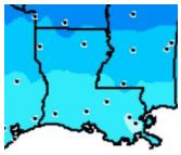
Wind Chill Days and Hours
(1973-2023)Midwest Regional Climate CenterThis set of maps depicts the average number of days, days with three or more hours, and the average number of hours per year with wind chill values at or below various thresholds (e.g., 15°F, 0°F, -10°F).
1. Near the top of the page, click on the map link of interest out of the three options: Average Number of Days, Days with 3 or More Hours, or Average Number of Hours. 2. Right above the map, mouse over the wind chill temperature value of interest to view the corresponding data on the map. 3. To interpret the colors, see the legend on the upper right side of the map. 4. To view more detailed information, such as station data, click the GIS Maps button on the top right of the page.
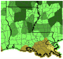
Freeze Maps
(1990-2020)Midwest Regional Climate CenterThis tool shows the average date(s) of the earliest fall freeze and latest spring freeze. The maps can be used to understand the times of the year in which you might experience temperatures below freezing for your area.
1. Click 28°F (or 32°F) FREEZE CLIMATOLOGIES on the left-hand side of the page to view the average dates of first/last freezes. Click any of the subcategories to view earliest, first, median, late, or latest freeze information. 2. Click on your area of interest on the map to zoom in to a parish-level view. Note: To only view station points on the map and remove the shaded regions, click Show Only Points (no shading) at the top of the page. 3. To view an interactive map with station information, click All Frost/Freeze Products at the top right of the page, then choose GIS Freeze Maps Interface.
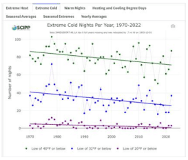
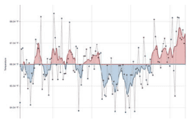
Temperature Trends Dashboard
(1970-2023) Southern Climate Impacts Planning ProgramThis tool shows temperature trends at individual stations across Louisiana, including trends in extremely cold nights, seasonal extreme and average high/low temperatures, and heating degree days, since 1970.
1. At the top of the tool, click the Extreme Cold, Heating and Cooling Degree Days, Seasonal Averages, or Seasonal Extremes tab. 2. The default station is in Abilene, TX. To choose a station nearest to you, use the map on the right. Zoom in and click any of the blue dots to change stations. You can also select a station under the Station drop-down menu on the left of the page 3. Use the graph to determine the trend (if any) for your selection. Solid lines represent significant trends. 4. Mouse over individual data points to view more information. 5. For seasonal selections, make sure Winter is selected in the Season drop-down menu on the left of the screen
Climate Change Trends
In recent decades, the number of days below freezing has declined across Louisiana, and the number of extremely cold days is expected to decrease (Frankson et al. 2022; Carter et al. 2018). Extreme cold events will continue to impact Louisiana; however, they are expected to occur less frequently and with less intensity (Frankson et al. 2022; Vose et al. 2017). Warmer winters signify that temperatures will remain warm for a longer amount of time, shortening the cold season which will subsequently lead to a longer freeze free period and growing season. By the end of the century under a high emissions scenario, the freeze-free season is projected to increase by more than one month in the southeast U.S., affecting ecosystems and agriculture (Carter et al. 2018). Also, by mid-century, the coldest day of the year is projected to be about 2-6°F warmer under a high emissions scenario in Louisiana (Vose et al. 2017). Read more about future cold extremes in Climate Change Science and Projection Resources.
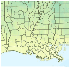
Climate Explorer – Climate Maps and Graphs Tools
(1950-2099)NOAA Climate Program Office and National Environmental Modeling and Analysis CenterThe Climate Explorer is an interactive tool that allows you to view and compare the annual heating degree days and the average number of days per year with a maximum or minimum temperature below 32°F for the historical period and in the future under both higher and lower emissions scenarios.
1. Type in the city or county you are interested in. 2. Click Climate Maps. 3. Using the drop-down menu in the upper-left corner, select the variable of interest (Days w/ max temp <32°F, Days w/ min temp <32°F, or Heating Degree Days). 4. Next to the drop-down menu, select Map. 5. Use the middle slider on the map to compare averages between the historical period (1961-1990) and future decades (2020s-2090s) under lower and higher emissions scenarios. (Use the bottom drop-down menus to choose variables and the slider on the bottom right to choose a decade to compare with.) On the map, zoom in to the county level and click a county to view the associated values. 6. To view this information over time (1950-2099) for a single location, click the Graph tab at the top of the map and type a location at the top.
Drought
Data Limitations
Drought cannot be assessed by a single indicator. Unlike many other hazards where impacts are immediate and apparent, drought has a slow onset and affects different sectors on different timescales. Consequently, it is important to assess drought using a variety of indicators, some of which respond better to short-term conditions, such as for agriculture, and others that respond to longer-term conditions, such as water resources. Many indicators are combined into the weekly U.S. Drought Monitor, however, this only dates back to 2000.
Definition and Description
A deficiency of moisture that results in adverse impacts on people, animals, or vegetation over a sizeable area (NWS 2009).
Drought impacts vary based on the duration and intensity of the event. A few dry weeks may affect crops and lawns, while droughts lasting months or years may significantly impact large water resources. At its extreme, nearly decade-long droughts may lead to farm and business foreclosures and mass migration. Some conditions that may lead to drought development include a large-scale, stationary high-pressure system which inhibits precipitation, feedback from dry soils accelerating warming of the air, La Niña which displaces jet streams, or large-scale ocean circulations in the Pacific and Atlantic Oceans. Droughts may happen in any location and at any time of year. Impacts often become severe more quickly for drought occurring during the summer, when evaporative loss is high; however, slower-evolving droughts in the fall and winter can have tremendous economic impacts on winter crops and livestock. Droughts are more frequent in areas where annual evaporation may exceed annual precipitation.
Drought is rated by the weekly U.S. Drought Monitor (2018) on a scale from D0 (abnormally dry) to D4 (exceptional drought). D0 occurs, on average, in any given location about 21-30% of the time. D1, moderate drought, occurs on average 11-20% of the time, or roughly once every 5-10 years. D2, severe drought, occurs 6-10% of the time, or about every 10-20 years. D3, extreme drought, occurs 3-5% of the time and D4, exceptional drought, occurs 0-2% of the time, or about every 50 years. Severity is based upon a variety of drought indicators, impacts, and input from local experts.
Historical Data
U.S. Drought Risk Atlas
(Period of record varies by station; up to ~130 years) National Drought Mitigation CenterThis interactive tool provides historical drought indices at a local level and can identify drought periods at different levels of severity, duration, and frequency.
1. On the left side, select Louisiana to search by state or zoom in on the map, then search by location. 2. Scroll down to select a station from the Station List on the right or choose a station from the map. Then, click Update Selection. 3. Below are a variety of drought indicator tabs to explore. Choose which indicator you would like to view. 3a. The Precip & Temp tab provides weekly, monthly, or annual averages of total precipitation and minimum and maximum temperature, shown in graphs. Select a date range or select a decade or the period of record from the drop-down menu. Select weekly, monthly, or annual information from the Aggregate drop-down menu. Choose to view a Time Series, Table, or Analog Ranks (top 10 information). 3b. The Drought Monitor tab shows values from the U.S. Drought Monitor, which began in 2000. Select a date range and a Boundary (state, parish, etc.). There are three ways to view the information. Select Time Series to view a graph of U.S. Drought Monitor values over time, averaged over the boundary you selected, Table to view a table of weekly drought monitor values, or Heat Map to view weekly values by year (use the slider to scroll through the weeks). 3c. The Trends tab shows various trends in several drought indicators and how statistically significant those trends are. Under the Index drop-down menu, select precipitation or a drought indicator. For any indicator, select a Start Year and Significance level. Some indicators require you to also select a Season, and the Precipitation indicator requires a Precipitation Threshold in inches. After you make the selections, click Trends Chart on the right. A graph will display the trend in the selected indicator over time. A blue dashed trendline represents an increasing trend in that indicator, a red dashed trendline represents a decreasing trend, and a black dashed trendline represents no trend. The trend value per decade is shown in text underneath the graph. Note: There are many other tabs with additional data and information. We only include a few prominent features here due to the complexity of other indices and length of instructions.
Historical Climate Trends Tool
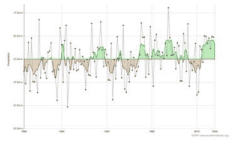
(1895-present) Southern Climate Impacts Planning ProgramThis interactive graphing tool shows precipitation trends, of which very dry periods are a drought indicator.
1. In the left column, moving from top to bottom, select Louisiana→ Climate Division of Interest → Season of Interest → Precipitation. 2. Hovering the curser over a point will display the year and total rainfall for the selected season. 3. For more information on how to interpret the chart, click on Chart Info on the bottom left.
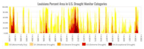
U.S. Drought Monitor Time Series
(2000-present) National Drought Mitigation CenterThis interactive graphing tool shows the frequency of drought conditions since 2000, along with each drought’s maximum intensity and duration (shown by color scale). The U.S. Drought Monitor is the official source for aid decisions by the USDA and several other agencies and programs.
1. In the top banner, next to Area type choose State, Climate Division, or County (parish). 2. Next to Area, select LA if you chose state-level information, or type a climate division or parish of interest. You can also type LA to view a drop-down list of all LA climate divisions/parishes. 3. Next to Index, select USDM. 4. Zoom in by clicking inside graph and dragging over a specific time-period.
Climate Change Trends
Louisiana has historically experienced droughts, but they have not been as long and intense as those further west, such as in Oklahoma and Texas. However, droughts are projected to increase in severity and frequency due to rising temperatures and increased evapotranspiration across the Southeast (Wehner et al. 2017; Carter et al. 2018). Even under a low emissions scenario, temperatures in Louisiana are projected to increase 1.5 °F by 2050 and 3°F by the end of the century in Louisiana (Frankson et al. 2022). Although summertime precipitation is not projected to change much in Louisiana, higher temperatures during dry periods will decrease soil moisture and exacerbate naturally occurring droughts (Frankson et al. 2022). Drought can increase wildfire risk, agricultural and economic losses, and stress to ecosystems (Carter et al. 2018). Read more about future drought in Climate Change Science and Projection Resources.
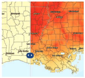
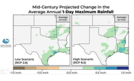
Precipitation Projections
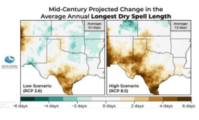
(2036-2099) South Central Climate Adaptation Science CenterThis webpage includes several precipitation projections, including the projected average annual number of days with rain and longest dry spell length, for the south-central U.S. for the mid-century (2036-2065) and end-of-century (2070-2099) time frames under low and high emissions scenarios.
1. The projections are grouped by mid-century and end-of-century. Scroll down to Projected Change in the Average Annual Number of Days with Rain or Projected Change in the Average Annual Longest Dry Spell Length for the time frame you’re interested in. These two variables relate to drought from a precipitation perspective. 2. The maps in the middle of the page show the projections under a low emissions scenario on the left and high emissions scenario on the right. The average value in the top right of each map represents the average for the entire region, so use the legend below the map to estimate the value for your area. Note: Click the map to view a larger version. 3. On either side of the page is a text summary of the projections for both emissions scenarios. Note: You can use these maps to view the range of projected values, as the future value will likely fall somewhere in between the low and high emissions scenarios.
Hail
Data Limitations
Hail data are not of sufficient quality to robustly determine historical trends and are of poorer quality than the tornado dataset. This is attributed to the increases in non-meteorological factors such as population and storm spotter coverage over time and the uncertainty in reported hail size. However, the recent decision to assess the number of hail days instead of individual hail reports has mitigated some biases. Also, note that the criteria for severe hail changed from 0.75” to 1” in 2009.
Definition and Description
Showery precipitation in the form of irregular pellets or balls of ice more than 5mm (0.2 inches) in diameter, falling from a cumulonimbus cloud (NWS 2009).
Hail forms by the collision of supercooled drops – raindrops that are still liquid even though the air around them is below freezing. The hailstone grows, supported by the updraft, until it is too heavy to remain aloft. Stronger updrafts generally produce larger hail size. Because obtaining large hail sizes requires a strong updraft, the timing of large hail is related to the lifecycle of large cumulonimbus clouds, which peak in intensity during late afternoon and evening hours. Updrafts may also be supported by vertical motion along a boundary, such as a front or mountains.
Hail severity is rated by the diameter of the largest hailstones in a storm. Hail of 1-inch diameter or greater is considered severe.
Historical Data
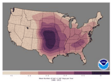
Severe Hail Days Per Year
(1986-2015)NOAA/National Weather Service Storm Prediction CenterThis map shows the average number of days per year in which severe hail reports occurred in the specified area during the period noted. The map provides a sense of the approximate number of days each year that you can expect to see severe (0.75- and 1-inch) or significant (greater than 2-inch) hail in your area. Note: Severe hail size changed from 0.75” to 1” in 2009, so both sizes are included on the webpage.
1. Scroll down and click on Hail Climatology – New Severe Hail (Greater Than 1.00” or Greater Than 2.00”) to view the full-size image.
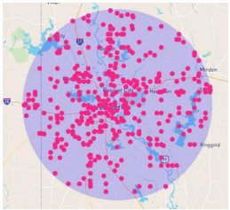
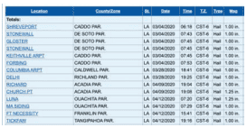
Severe Hail Reports
Hail: (1955-present) Southern Regional Climate CenterThis interactive tool displays the historical record of individual severe hail reports in your area. It can be used to determine hail events that have impacted your area.
1. On the left side of the screen, click on Search within Radius. 2. Choose the diameter of the area you want to investigate (25 or 50 miles). 3. Pan, zoom, and then click on the map area of interest. 4. Under Filter by Storm Types select Hail (de-select all other storm types). 5. Reports are displayed on the map and in two tables below the map.
Map: Mouse over individual storm reports for details.
Tables: There are two tables, Recent Storm Data and Historical Storm Data. Click on a column header to sort by column of interest. For example, to view the dates on which the largest hail occurred, click on the Scale column headers to sort by the largest hail values.
Storm Events Database
Hail: (1955-present) NOAA National Centers for Environmental InformationThis interactive tool displays the historical record of individual severe hail reports by parish. It can be used to determine hail events that have impacted your area or close to your area.
1. On the bottom left, under Select State or Area, choose Louisiana → Search 2. From top to bottom, select a specific Begin and End Date, and Parish of interest. 3. Under Event Type(s), select Hail. 4. Expand Advanced Search and Filter Options → Hail Filter, select hail size of interest. 5. Press Search. Summary results are presented in a table. Note: This tool can be used to analyze a variety of additional hazards with various time periods, and hail data goes as far back as 1955. This database is likely incomplete and does not account for all hail events.
Climate Change Trends
Hail is commonly associated with severe thunderstorms, and Louisiana has experienced at least one day per year with hail larger than 1 inch from 1986-2015. Northern Louisiana experiences 1-inch or larger hail, on average, 3-4 days per year (SPC 2016). Climate models project an increase in the atmospheric conditions that tend to favor severe thunderstorms, especially events capable of producing large hail (Kossin et al. 2017). Confidence in the projections is low, however, due to the isolated and sporadic nature of hail events and limited comprehensive datasets that make it difficult to track long-term trends (Wuebbles et al. 2017a).
Heat Extremes
Data Limitations
Louisiana generally has high quality long-term data records for temperature; however, the consistency of cumulative years on record varies by station. Additionally, some station locations include gaps in records that could be subject to technical issues or changes in monitoring location.
Definition and Description
A heat wave is an occurrence of unusual hot weather (maximum, minimum, and daily average) over a region persisting at least two consecutive days during the hot period of the year based on local climatological conditions, with thermal conditions recorded above given thresholds (WMO 2016).
Note: There is no universally recognized metric for what constitutes a heat extreme. The World Meteorological Organization recommends characterizing a heat wave by its magnitude, duration, severity, and extent. Magnitude is defined as a thermal measurement such as maximum temperature, or combination of several measurements, exceeding certain threshold(s). These values must be determined by the local climatology. Other studies have used thresholds based on human physiological response to heat, such as consecutive days of maximum or minimum temperatures above a threshold.
Heat extremes in the central United States occur when a dominant large-scale high-pressure system prevents the movement of other air masses into a region. The high-pressure contributes to intense heating from solar radiation, due to a lack of cloud cover, and light winds preventing the dispersion of heat, especially from urban areas. This results in both higher than average maximum and minimum temperatures.
Historical Data
Historical Climate Trends Tool
(1895-present) Southern Climate Impacts Planning ProgramThis interactive graphing tool shows annual, seasonal, and monthly temperature trends by state and climate division. It can be used to gain a general understanding of temperature trends and show previous periods of higher temperatures and years of extreme temperature.
1. On the left side of the screen (from top to bottom) select Louisiana → Climate Division of Interest (or leave as Entire State) → Season of Interest → Temperature. 2. For more information on how to interpret the chart, click on Chart Info.
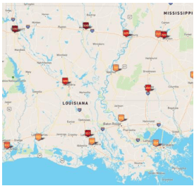
Climate Extremes Tool - Temperature
(Period of record varies by station; up to ~130 years) Southern Regional Climate CenterThis interactive tool shows temperature extremes at point locations. It can be used to show the severity of past events in a region of interest. Highlighted below are two ways the tool can be used to analyze heat extremes:
(a) High temperature records by month: 1. On the left side of the screen (from top to bottom) select Records For A Month → High Max Temperature → Month of Interest → Submit. 2. Mouse over icons for record details including station name, date of occurrence, and station period of record.
(b) All-time records: 1. Select All-Time Records → High Max Temperature→ Submit. 2. Mouse over icons for record details including station name, date of occurrence, and station period of record. Note: For more information, select the Help or About tabs.
Heat Index Days and Hours
(1973-2023)Midwest Regional Climate CenterThis set of maps depict the average number of days, days with three or more hours, and the average number of hours per year with heat index values at or above a variety of thresholds (e.g., 95°F, 105°F, 110°F).
1. Near the top of the page, click on the map link of interest out of the three options: Average Number of Days, Days with 3 or More Hours, or Average Number of Hours. 2. Right above the map, mouse over the heat index value of interest to view the corresponding data on the map. 3. To interpret the colors, see the legend in the upper-right corner of the map. 4. To view more detailed information, such as station data, click the Interactive GIS Maps button on the top right of the page.
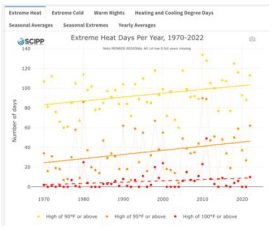
Temperature Trends Dashboard
(1970-2023)Southern Climate Impacts Planning ProgramThis tool shows temperature trends at individual stations across Louisiana, including trends in extremely hot days, warm nights, seasonal extreme and average high/low temperatures, and cooling degree days, since 1970.
1. At the top of the tool, click the Extreme Heat, Warm Nights, Heating and Cooling Degree Days, Seasonal Averages, or Seasonal Extremes tab. 2. The default station is in Abilene, TX. To choose a station nearest to you, use the map on the right. Zoom in and click any of the blue dots to change stations. You can also select a station under the Station drop-down menu on the left of the page. 3. Use the graph to determine the trend (if any) for your selection. Solid lines represent significant trends. 4. Mouse over individual data points to view more information. 5. For seasonal selections, make sure you select a season in the Season drop-down menu on the left of the screen.
Climate Change Trends
The frequency and intensity of heatwaves and extreme heat events have increased across the U.S. since the mid-1960’s (Wuebbles et al. 2017b). As the global temperature continues to increase, the occurrence and intensity of extreme heat events are projected to increase. The warmest temperature of the year could rise by up to 6°F across Louisiana by the middle of the century (Vose et al. 2017). Furthermore, the number of days above 90°F may increase by 40-50 days per year for this time frame and scenario as well. Combined with the humidity that Louisiana experiences, this can lead to increased heat stress to people and animals. There has also been an increasing trend in warm nights, further exacerbating heat stress by preventing people and animals from getting nighttime relief from the heat (Frankson et al. 2022). Read more about future heat extremes in Climate Change Science and Projection Resources.
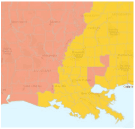
Killer Heat Tool
(1971-2099) Union of Concerned ScientistsThis interactive mapping tool shows the number of days with a maximum heat index above 90°F, 100°F, 105°F, and ‘off the charts’ (exceeding the upper limits of the NWS heat index scale) for each U.S. county/parish over the historical baseline (1971-2000), mid-century (2036-2065), and late-century (2070-2099). Future projections include scenarios for no action, slow action, and rapid action on climate change.
1. At the top of the tool, click the Above 90, Above 100, Above 105, or Off the Charts tab. 2. Zoom in to the desired area on the map. The default map displays the historical number of days above the threshold. 3. Click the parish of interest to view the historical number of days per year above the selected heat index threshold. 4. On the left panel, scroll through the text and select a future scenario with no action on climate change, with slow action on climate change, or with rapid action on climate change for the Midcentury or Late Century time frame. 5. Click the parish of interest to view the number of days per year above the selected heat index threshold for the scenario and time frame selected. 6. This information is also available for military bases in the U.S., accessible through the Military Bases at Risk tab at the top of the page.
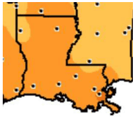
Climate Explorer – Climate Maps and Graphs Tools
(1950-2099) NOAA Climate Program Office and National Environmental Modeling and Analysis CenterThe Climate Explorer is an interactive tool that allows you to view and compare the average number of warm nights, extremely hot days, and cooling degree days per year for the historical period and in the future under both higher and lower emissions scenarios.
1. Type in the city or parish you are interested in. 2. Click Climate Maps. 3. From the drop-down menu, select Days w/ max temp > 90 (or other option up to 105°F), Days w/ min temp > 80°F (or 90°F), or Cooling Degree Days 4. Next to the drop-down menu, select Map. 5. Use the middle slider on the map to compare averages between historical, lower, and higher emissions scenarios. (Use the bottom drop-down menus to choose variables and the slider on the bottom right to choose a decade to compare with.) On the map, zoom in to the parish level and click a parish to view the associated values. 6. To view this information over time (1950-2099) for a single location, click the Graph tab at the top of the map and type a location at the top.
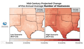
Temperature Projections - Heatwaves
(2036-2099) South Central Climate Adaptation Science CenterThis webpage includes several temperature projections, including the projected number of heatwaves per year, for the south-central U.S. during the mid-century (2036-2065) and end-of-century (2070-2099) time frames under low and high emissions scenarios.
1. The projections are grouped by mid-century and end-of-century. Scroll down to Projected Change of the Annual Average Number of Heatwaves for the time frame you’re interested in. The maps in the middle of the page show the projections under a low emissions scenario on the left and high emissions scenario on the right. The average value in the top right of each map represents the average for the entire region, so use the legend below the map to estimate the value for your area. Note: Click the map to view a larger version. 3. On either side of the page is a text summary of the projections for both emissions scenarios. Note: You can use these maps to view the range of projected values, as the future value will likely fall somewhere in between the low and high emissions scenarios.
Heavy Rainfall and Flooding
Data Limitations
There is a relatively long historical record of precipitation data. However, there can be gaps between station locations, so some rainfall events, including high rainfall amounts, may not be adequately represented in the data. Also, flood risk depends on a precipitation event, preceding events, the built environment, and flood mitigation techniques. Flooding can and does occur outside of the Federal Emergency Management Agency (FEMA) Special Flood Hazard Areas. Flood impacts are often extremely localized, so the data listed below may not adequately represent a single community or neighborhood flood risk or history.
Definition and Description
Heavy rainfall is rain with a rate of accumulation exceeding a specific value that is geographically dependent (AMS 2012). Flooding is any high flow, overflow, or inundation by water which causes or threatens damage (NWS 2009).
Heavy rainfall is a subjective term, but is rain falling at a rate more than the underlying surface can handle, causing runoff, inundation of low-lying areas, and flooding. This may include short-duration thunderstorms lasting a few hours or rainfall accumulating over several days. Flooding is the result of heavy rainfall but also the underlying surface. The rate of infiltration (how quickly it is absorbed by the soil), how quickly runoff reaches the creeks and rivers, if there had been prior rainfall, if the ground is frozen, and other local factors affect runoff and flooding. Consequently, a rainfall of a given rate and amount may cause flooding in one circumstance but not in another. Flooding is most likely in low-lying areas, along the edges of water bodies (ponds, lakes, rivers), and over impermeable surfaces (such as streets and parking lots). Primary causes include slow-moving thunderstorms and storms that track over a location in rapid succession, or tropical systems. Flash flooding may occur with intense thunderstorms while river flooding usually requires rainfall accumulated over a longer duration.
Rainfall accumulations may be compared against previous occurrences through the concept of “return-period values”. This is a statistical assessment of the frequency with which similar amounts have been recorded in the past at a specific location. These return periods, such as 1 in 25 years (a 4% chance of occurring in any given year), are not predictive tools – a large event occurring in the recent record does not prevent another similar or larger event occurring shortly after. Also, if heavy rainfall has already occurred, stormwater retention systems may be filled to capacity allowing a smaller event to cause flooding impacts similar to a much larger event. Rainfall rates and accumulations are usually greatest during the spring, summer, and fall, when warm air can hold more water vapor to produce greater rain rates. River flooding is most likely in spring or fall, when fronts may stall giving a focus for thunderstorm development. Tropical systems, either from the Gulf of Mexico or from the Pacific Ocean, can produce among the highest rainfall rates in the state.
Historical Data
Climate Extremes Tool – Precipitation
(Period of record varies by station; up to ~130 years) Southern Regional Climate CenterThis interactive map shows daily precipitation extremes at airport weather stations, which can be used to show some previous heavy rainfall occurrences (i.e., the highest rainfall totals do not necessarily occur at airport weather stations).
1. Pan and zoom to the location of interest. 2. To obtain High precipitation records by month: On the left side of the screen, select Records For A Month → High Precipitation → Month of interest → Submit. 3. The measurement unit is inches. Mouse over the icon on the map for record details (date of occurrence and station record). 4. To obtain All-time records: Select All-Time Records → High Precipitation → Submit.

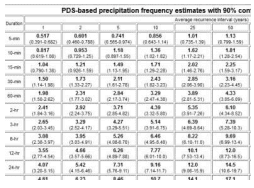
NOAA Atlas 14 Precipitation Frequency Data Server
(Last updated in 2013) NOAA Hydrometeorological Design Studies CenterThis interactive tool shows rainfall frequency estimates for select durations (e.g., 3-, 12-, and 24-hours) and recurrence intervals (e.g., 100-, 500-, and 1000-years) with 90% confidence intervals. Probable maximum precipitation (PMP) values are not represented in this tool.
1. Click on Louisiana from the map. A new tab will open. 2. To select a location, either enter the desired location, station, or address manually OR double-click the interactive map. 3. Precipitation frequency estimates will be displayed in both table and graph forms below. 4. For additional help, select FAQ from the left-hand menu, then refer to the Section 5 link under section 1.1.
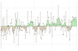
Historical Climate Trends Tool
(1895-present)Southern Climate Impacts Planning ProgramThis tool shows precipitation trends by state and climate division, annually, seasonally, and monthly. Years, seasons, or months with high precipitation totals may be indicative as years with flood events during one or more parts of the year, however, this must be correlated with other data.
1. On the left side of the screen, select Louisiana. 2. Select the climate division of interest or the entire state. 3. Select annual, season, or month of interest. 4. Select Precipitation. 5. For more information on how to interpret the chart, click on Chart Info on the bottom left and hover over points to view individual precipitation values.
Climate Explorer – Historical Thresholds Tool
(Period of record varies by station; up to ~130 years) NOAA Climate Program Office and National Environmental Modeling and Analysis CenterThe Climate Explorer is an interactive tool that allows you to view the number of extreme rainfall events per year for a station’s period of record, among many other features.
1. Type in the city or county you are interested in. 2. Click Historical Thresholds. 3. From the top menu, select a Threshold in inches (e.g., 1 in). 4. Select a duration Window in days (e.g., 1 day). 5. Choose a station (red dot) on the map. 6. The resulting plot displays a bar chart with days per year (or multi-day duration you chose) with precipitation reaching your selected threshold. Hover your mouse over the bars to view yearly information.
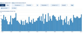
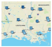
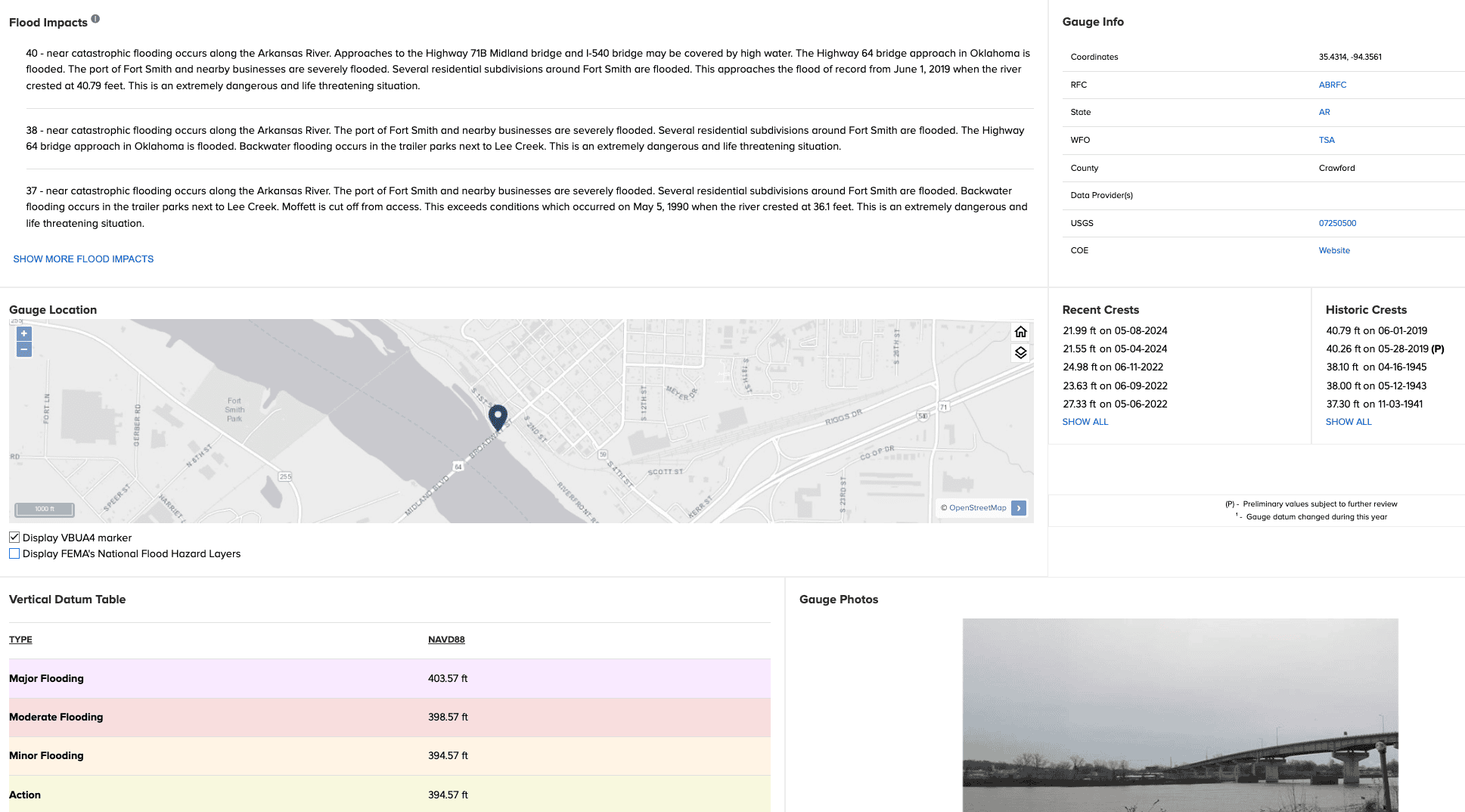
Flood Impacts by River Crest Height
(Period of record varies by gauge; up to ~110+ years)NOAA National Weather ServiceThis interactive tool shows a summary of flood impacts and historical gauge information for locations of interest. It can be used to identify historic and recent river crest heights, flood impacts by crest height and location, and hydrographs.
1. On the map, pan and zoom to the area of interest. Click on the stream gauge of interest on the map. 2. A new side window will pop up with the selected gauge’s information. Click Full Information at the top. 3. A hydrograph with recent and forecasted values is shown at the top. Below this is a table with flood stages and associated crest heights. To view Flood Impacts for a range of crest heights, scroll down the page. Click Show More Flood Impacts to expand this list. 4. Recent Crests and Historic Crests are listed below and to the right. These lists show the crest height and date of the observation. 5. Below this is the Vertical Datum Table with associated flood stages.
FEMA Flood Map Service Center
Federal Emergency Management AgencyThis website can locate and identify flood hazard zones in a jurisdiction and produce maps for use in a hazard mitigation plan. Combined with other map layers, it can provide a spatial relationship between flood hazard zones and critical facilities and infrastructure. Note that the 100-yr floodplain is an estimate used for insurance and regulatory purposes. Floods can and do occur outside of the areas depicted. Note: This tool is a little more involved than some of the others and it is helpful to use a larger computer screen because of the amount of data shown.
1. Enter an address, place, or coordinates in the search bar. 2. Click Search. 3. Click Streets view in upper right corner. 4. The panel of land outlined in light blue is what will be mapped. If you need another panel, click on the one of interest. (Zoom out if needed. It may take a few seconds.) 5. Zoom in to view details. Note the legend below the map and effective date in bold above the map. 6. To download a black and white static image of full original FIRM panel, click on the Map Image icon. To access a colored map, click on the Dynamic Map icon. You may need to disable your browser’s pop-up blocker.
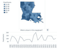
Historical Flood Risk and Costs
(1996-2019) Federal Emergency Management AgencyThis map visualization and graph shows state and parish flood events that are documented in NOAA’s Storm Events Database. It shows the number of flood events by parish and costs of flooding based on average National Flood Insurance Program and FEMA’s Individual and Household Program payments.
1. Under Choose a State, select Louisiana. 2. Louisiana statistics will be displayed on the page. 3. If you wish to view statistics by parish, click on a parish on the map.
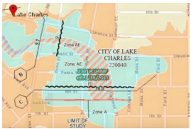
Louisiana FloodMaps Portal: The Base Flood – on the map
LSU AgCenter, LA Dept. of Transportation & DevelopmentThis tool provides information about flood risk at a particular location and shows how FEMA’s Flood Insurance Rate Maps (FIRM) have changed over time.
1. Click Continue. 2. Enter an address/coordinate or select a parish from the drop-down menu. Note: if you select a parish, the page may bring you back to the welcome page. If so, just click Continue again, then click the X to exit the location pop-up menu on the mapping page. 3. The map shows the Effective FIRM, floodway areas, and other layers. 4. Click the Layers button on the top right to select various FIRM layers and ABFE (Advisory Base Flood Elevation; if available). Click the question mark next to any layer to read more. 5. Click the Legend button on the top right to interpret all map features. 6. Zoom in and click on the map for point-specific information. On the resulting pop-up box, click Community Info or What Does This Mean? to learn more. Note: Click the “i” on the top right of the screen for additional guidance.
FEMA's Estimated Base Flood Elevation Viewer
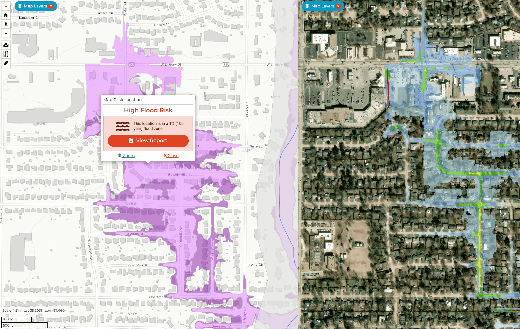
Federal Emergency Management AgencyThis tool shows Base Level Engineering datasets, models, maps, and reports that allow users to visualize and download flood risk data for their community and give property owners site-specific flood risk information. This helps them understand the possible risk to their homes and businesses and make informed decisions to reduce damage from future floods.
1. In the Select an Area of Interest drop-down menu, select FEMA Region 6. 2. On the next screen, select What’s My Flood Risk? to view a local report with estimated base flood elevation (BFE). 3. A panel of two maps is on the next page: 1% (100-year) and 0.2% (500-year) flood extent on the left and flood depth (1%) on the right. To quickly produce a BFE report, follow the options on the left menu under the Report tab to either enter a location of interest, click a location on the map, or use your current location. Note: A report will only generate when BFE data are available at that location. To view where data are available, zoom in on the map and click a property that is in the 1% flood extent area (purple color on the left map; click Legend next to the Report button on the top left to view the legend). If BLE data are unavailable, a pop-up box will notify you when you click a location. If the property is in a study zone (gray area), the tool will direct you to another tool and will not produce a report. 4. After selecting a location, click View Report. A new page shows the 2-page report with estimated flood extent, flood depth, and base flood elevation. The second page includes more information about using the data and taking action.
5. To explore the map, go back to the BFE Viewer tab on your web browser. Click the Legend tab at the top left of the page. 6. On each map, click Map Layers to choose other data to explore. In the Base Level Engineering drop-down menu, you can select other flood extents or depths, as well as other information. You can view only one map at a time by clicking 1 Map View on the top right of the screen.
Climate Change Trends
Total annual precipitation has largely been above average in Louisiana since 1970, and the frequency of 4-inch extreme precipitation events have been above average since 1980 (Frankson et al. 2022). Across Louisiana, the intensity of hourly rainfall has increased over time (Brown et al. 2019). While annual precipitation amounts are not projected to change much, heavy precipitation events may increase in frequency and intensity (Hayhoe et al. 2018). By the end of the century, the heaviest 1% of rainfall events are projected to increase by up to 40% in intensity under a higher emissions scenario in northern Louisiana and up to 20-30% in southern Louisiana (Hayhoe et al. 2018). With the possibility of more intense rainfall from tropical storms and increased sea level rise and subsidence, flooding risks further increase in coastal and low-lying areas of Louisiana. Intense rainfall, including from tropical storms, has already increased by 6-7% compared to a century ago (Hayhoe et al. 2018). Flooding can cause overflow of sewage systems and contaminants of water resources, displacement of communities, disruption of critical services, and more. Read more about future heavy rainfall events in Climate Change Science and Projection Resources.
Risk Factor
(Present risk and 30- year future projections) First Street FoundationThis tool provides information on flood risk and how it is changing. It shows the trend in number of properties at risk, a specific property’s flood risk score, the flood history of an area, and how an area’s flood risk is expected to change.
1. Type in the county, city, or zip code of interest. 2. Click the Flood Factor tab near the top of the page. 3. Scroll down the page to view flood risk information. Note: Many features on this tool are behind a paywall. If you want information for specific homes and businesses or want to dive deeper into the information, then payment is required. However, you can receive the baseline information above for free.
Climate Explorer – Climate Maps and Graphs Tools
(1950-2099) NOAA Climate Program Office and National Environmental Modeling and Analysis CenterThe Climate Explorer is an interactive tool that allows you to view and compare the average number of days with precipitation greater than 1”, 2”, or 3” per year for the historical period and in the future under both higher and lower emissions scenarios.
1. Type in the city or parish you are interested in. 2. Click Climate Maps. 3. From the leftmost drop-down menu, select Days w/ 1” Precipitation (2” and 3” thresholds are also available). 4. Next to the drop-down menu, select Map. 5. Use the middle slider on the map to compare averages between historical, lower, and higher emissions scenarios. (Use the bottom drop-down menus to choose variables and the slider on the bottom right to choose a decade to compare with.) On the map, zoom in to the parish level and click a parish to view the associated values. 6. To view this information over time (1950-2099) for a single location, click the Graph tab at the top of the map and type a location at the top. Note: Precipitation projections have a high range of uncertainty.
Precipitation Projections
(2036-2099) South Central Climate Adaptation Science CenterThis webpage includes several precipitation projections for the south-central U.S. during the midcentury (2036-2065) and end-of-century (2070-2099) time frames under low and high emissions scenarios.
1. The projections are grouped by mid-century and end-of-century. Scroll down to Projected Change in the Average Annual 1-Day (or 5-Day) Maximum Rainfall for the time frame you’re interested in. 2. The maps in the middle of the page show the projections under a low emissions scenario on the left and high emissions scenario on the right. The average value in the top right of each map represents the average for the entire region, so use the legend below the map to estimate the value for your area. Note: Click the map to view a larger version. 3. On either side of the page is a text summary of the projections for both emissions scenarios. Note: You can use these maps to view the range of projected values, as the future value will likely fall somewhere in between the low and high emissions scenarios.
High Tide Flooding
Data Limitations
The tide-gauge network is sparse, so there is a lack of tide data for many coastal communities and inconsistent periods of record for locations with gauges. Tide gauges are often placed in harbors and locations with protective housing that can reduce wave effects, preventing measurements of higher-frequency wave effects (Sweet et al. 2022). There is not a long-term record in many areas, and models that increase data coverage often underestimate water levels in areas with frequent tropical storms (Muis et al. 2016).
Definition and Description
Flooding that leads to public inconveniences such as road closures, occurring when tides reach anywhere from 1.75 to 2 feet above the daily average high tide and start spilling onto streets or bubbling up from storm drains (NOS 2021; NOAA 2022).
Coastal flooding may occur during high tides, even without a strong storm or hurricane. The combination of sea-level rise, land subsidence, and the loss of natural barriers contributes to an increased frequency of flooding capable of closing roads and damaging property. High-tide flooding may also contribute to flooding away from the immediate coast when stormwater systems cannot drain, such as from a thunderstorm occurring during a high-tide event. The frequency of high-tide flooding along the coast has doubled over the past 30 years (NOS 2021).
High tides occur when the moon is in alignment with the sun, at either a new moon or a full moon phase. This causes slightly higher tides than at other days in the month. If ocean waters are particularly warm or there is a nearby storm system, this can add to high tide levels through thermal expansion or wind and pressure effects.
Historical Data
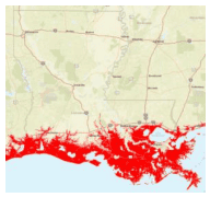
Coastal Flood Exposure Mapper
National Oceanic and Atmospheric AdministrationThis interactive mapping tool shows areas susceptible to high tide flooding, water depth from sea level rise, storm surge from different hurricane categories, and FEMA flood zones. Users can overlay societal, infrastructure, and ecosystem exposures.
1. Click Get Started. 2. Zoom in to the area of interest. 3. Click the layers icon in the bottom-left corner to change the map. 4. To view areas susceptible to high tide flooding, click the High Tide Flooding option under Hazard Layers. 5. Click any of the exposure layers, such as Critical Facilities, to add additional information to the map.
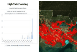
Sea Level Rise Viewer
(High Tide: 1980-present in Louisiana) National Oceanic and Atmospheric AdministrationThis mapping tool visualizes the impacts of sea level rise and allows users to choose different water levels to view sea level rise projections, overlay community vulnerability, and view high tide flooding frequency. Note: this tool only includes 1 tide gauge in Louisiana.
1. Click Get Started. 2. Zoom into the area of interest. The default map is the current water level, where darker blues are greater water depths. 3. Click High Tide Flooding on the lefthand menu. Red areas represent shallow coastal flooding areas and tide gauges are shown at select locations (you may have to zoom in to view these). 4. Click the tide gauge icon on the map to view a graph of yearly high tide flooding events per year at that location. Note: access the legend by clicking the middle icon on the top right of the screen.
Gulf Tree
(Time frame varies by product) Northern Gulf of Mexico Sentinel Site Cooperative, Gulf of Mexico Climate Resilience Community of Practice, & Gulf of Mexico Alliance Resilience TeamThis decision support site guides users to the high tide/nuisance flooding tools and resources they need along the Gulf Coast through several filters of information, including how much time and effort they are willing to spend on the tool.
1. Choose a Filtered Search to look through all filter categories on one page or choose Guide My Search to walk through questions step by step to achieve what you’re looking for. 2a. If you chose the Filtered Search, first navigate to Geographic Scope. Click the Louisiana drop-down menu and choose Shoreline to select all coastal parishes or choose specific one(s). 2b. Under Tool Function, select what you’d like to use high tide flooding information for. You can leave this blank if you’re unsure which to choose. 2c. Under Cost, choose Free. 2d. Under Level of Effort, choose from low, moderate, or high (will determine how advanced the tool is). 2e. Under Climate Change Topics, select the drop-down for Flooding, then check the box for Nuisance Flooding. Explore other drop-down menus in this section to add more filters for additional topics. 2f. Click View Tool Matches on the top right to go to the results page. Click any of the tools or resources to go to that site.
3a. If you chose Guide My Search, Gulf Tree will walk you through the same filters by asking 6 questions. For step 1 (Tool Function), check the box for why you need a high tide flooding tool, then click Submit. If you’re not sure which option to use, you can Skip this step. 3b. Step 2 (Topic Area) includes a filter for what aspect of the topic you’re interested in. Click the drop-down menu for Flooding and check the box for Nuisance Flooding, then click Submit. 3c. On Step 3 (Location), click the Louisiana drop-down menu, then choose Shoreline to select all coastal parishes or choose specific one(s). Then, click Submit. 3d. For Step 4 (Level of Effort), choose how much effort you’d like to put into the tool, which will determine how advanced the tool is. Then, click Submit. 3e. For Step 5 (Tool Cost), choose Free, then click Submit. 3f. Click Leave Guided Search and View Matches to go to the results page or go back to a previous page on the left menu to change your selected options. Click any of the tools or resources to go to that site. 6. To create a new search, click Reset All Filters at the top right of the results page.
Climate Change Trends
As sea levels rise, coastal flooding is expected to increase, causing more frequent high tide flooding events that reach further inland (Sweet et al. 2022). The 2022 NOAA Sea Level Rise Technical Report (Sweet et al. 2022) analyzed high tide flooding from the mean higher high water (MHHW), which is the average height of the highest tide recorded at a tide station each day during the recording period. By 2050, minor/disruptive high tide events (0.5 m above MHHW) are projected to occur more than twice as often than in 2020, and major/often destructive events (1.2 m above MHHW) may occur five times more often along the western Gulf Coast (Sweet et al. 2022). The U.S. coasts are experiencing a flood regime shift, in which high tide flooding events have increased, and only 1-2 feet of sea level rise will transition more “nuisance” flooding events to more moderate to major flooding events. Read more about future high-tide flooding in Climate Change Science and Projection Resources.
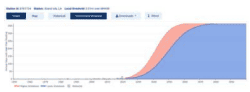
Climate Explorer – High-Tide Flooding Tool
(1950-2099) NOAA Climate Program Office and National Environmental Modeling and Analysis CenterThe Climate Explorer is an interactive tool that provides the annual number of days with high-tide flooding for the historical period (up to 1950-present) and modeled projections (present-2099) under a lower and higher emissions scenario.
1. Type in the city or parish you are interested in. Click High-Tide Flooding. 3. Click a station (blue dot) on the map. Note: there is only one station available in Louisiana, near Grand Isle. 4. The resulting graph shows the annual days with high-tide flooding. The gray bars represent historical observations and the curves from the present year through 2099 represent the modeled/projected values, where red displays the higher emissions scenario and blue shows the lower emissions scenario. 5. Hover your mouse over the graph to view the observed or projected values.
Hurricane/Tropical Storm/Storm Surge
Data Limitations
Tropical Cyclone (TC) data prior to the satellite era is limited since only land and ship observations were available. This can make it difficult to conclude whether TC activity is increasing or if it is due to better observation systems (Walsh et al. 2015). Similarly, there are gaps in storm surge data with older storms. Storm surge models do not handle leveed areas well, and modeling water levels under levee failure scenarios is complex.
Definition and Description
Hurricane: A tropical cyclone in the Atlantic, Caribbean Sea, Gulf of Mexico, or eastern Pacific, in which the maximum 1-minute sustained surface wind is 64 knots (74 mph) or greater (NWS 2009).
Storm Surge: An abnormal rise in sea level accompanying a hurricane or other intense storm, whose height is the difference between the observed level of the sea surface and the level that would have occurred in the absence of the cyclone. Storm surge is usually estimated by subtracting the normal or astronomic tide from the observed storm tide (NWS 2009).
Hurricane: A hurricane begins as a tropical cyclone, a disturbance that originates over warm ocean waters with organized deep convection and a closed surface wind circulation about a well-defined center. When sustained winds reach 34 knots (39 mph), it is classified as a tropical storm and at sustained winds greater than 64 knots (74 mph) it becomes a hurricane. Each tropical storm or hurricane is given a unique name to track its progress.
Hurricanes need warm ocean waters, an unstable atmosphere, a deep layer of moist air, a pre-existing surface disturbance, and very little vertical wind shear to form. They convert warm, moist air into energy that strengthens the circulation; consequently, when they move over land they weaken quickly. Hurricane season runs from June through December, with a peak around September 10. The Gulf of Mexico peak is usually a few weeks earlier because the shallower water warms faster than the deeper Atlantic Ocean.
Hurricane impacts include winds, storm surge, tornadoes, and inland flooding. Sustained winds over 160 mph with gusts over 200 mph may be recorded in the most intense hurricanes and can extend 30-600 miles away from the storm’s center. Tornadoes are often embedded within the rainbands swirling outward from the center and are most common in the right-front quadrant of the storm. Inland flooding may be caused by several feet of rain over a few days, especially for a slow-moving or stalled hurricane. Hurricane Harvey produced 60 inches of rain over a 5-day period.
Storm Surge: Storm surge is often one of the greatest threats to life and property from a hurricane. Storm surge is a very complex phenomenon because it is sensitive to the slightest changes in storm intensity, forward speed, size (radius of maximum winds), angle of approach to the coast, central pressure (minimal contribution in comparison to the wind), and the shape and characteristics of coastal features such as bays and estuaries. Higher wind speeds from a hurricane lead to increased storm surge. A slower-moving hurricane also leads to higher and broader storm surge inland while a faster-moving hurricane can lead to increased storm surge over open coastal areas. One cause of structural damage from storm surge is the extension of waves further inland that can include water weights of approximately 1,700 pounds per cubic yard. Storm surge can also cause coastal erosion, damaging beaches and coastal roads (NHC 2022a).
Storm surge is observed and measured by NOAA tide stations, FEMA/USGS high water marks, and temporary USGS pressure sensors. NOAA tide stations are a network of continuously operating water level stations throughout the U.S. serving as the foundation for NOAA’s tide prediction products and providing data for storm surge estimates. This data is traditionally the most reliable, but there are limited stations. FEMA/USGS high water marks (HWM) are lines found on trees and other structures marking the highest elevation (peak) of the water surface for a flood event created by foam, seed, or other debris. Survey crews are deployed after a storm to locate and record reliable HWMs. GPS methods are used to determine location for coastal HWMs, which are then mapped relative to a vertical reference datum such as NAVD88. This is traditionally the best method for capturing the highest storm surge level. USGS pressure sensors are temporary water-level and barometric- pressure sensors which provide information about storm surge duration, times of surge arrival/retreat, and maximum depths. These sensors are deployed in advance of an upcoming storm in an area in which the highest surge is expected (NHC 2022b).
Historical Data
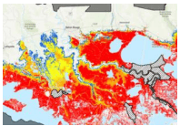
Coastal Emergency Risks Assessment
(2012-present) Louisiana State University, Louisiana Sea GrantThis tool allows users to view current, recent, and storm-specific water heights above Mean Sea Level and wind speed. For specific storms, you can also view the storm track and inundation depth above ground. Note: to access all features, you may need to sign up and request a free account.
1. Select a day or storm of interest at the top left. 2. Zoom into the area of interest to view sea level anomalies. 3. Use the options on the right of the screen to choose other variables to view.
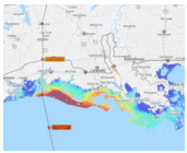
National Storm Surge Risk Maps
NOAA National Hurricane CenterThis mapper allows users to assess their storm surge risk at various hurricane intensities by displaying the maximum possible storm surge for each storm category. This tool can be used to assist in forming evacuation plans for both individuals and decisions makers.
1. Zoom to the area of interest. 2. Click through the different hurricane categories at the top of the page to view storm surge levels for that area at different hurricane strengths.
SURGEDAT: The World’s Storm Surge Data Center
(Time frame varies by product; up to ~140 years) Southern Climate Impacts Planning ProgramSURGEDAT is an extensive storm surge database for the Gulf of Mexico and East Coast. This site provides access to data and several storm surge tools. The following are active and open to the public:
Live Storm Updates and Archive: http://surge.climate.lsu.edu/
This page allows the user to choose a tropical storm/hurricane of interest and view the associated storm surge levels, sea level pressure, and wind speed and direction.
1. Select the current storm or click the archive link and select a past storm of interest. 2. A new page will open with a graph of storm surge levels at different station locations over the duration of the event and a map of the storm path and gauge locations. 3. Hover over the storm path on the map to view the wind speed and direction, moving speed, and pressure for points along the path of the storm.
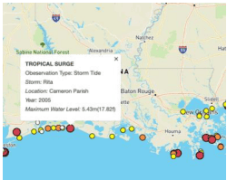
Global Peak Surge Map: http://surge.climate.lsu.edu/data.html#GlobalMap
This page allows the user to view the peak recorded storm surge at a location of interest since 1880.
1. Zoom and pan to an area on the map. 2. Click a dot to view peak surge information. 3. The box describes the observation type, associated storm, location name, year, and the max water level recorded at that location.
Interactive Surge Map: https://surgedat.climate.lsu.edu/surge/
This tool provides a table of storm surge history and graphs of return periods, storm surge heights by year, and ranking of storm surge heights for a selected area.
1a. Search by Storm: Choose a storm and then year from the drop-down menus. 1b. Click an icon on the map to view the peak storm surge/tide at that gauge for the selected storm. A list of the peak storm surge/tide values for each gauge are in the table below the map. 2a. Search by Location: Enter a latitude (top box) and longitude (bottom box) if known and choose a distance from that point. If the coordinates are unknown, then first choose a distance from the drop-down menu, then click the map to select your desired location. 2b. Graphs on the right provide information about return periods with associated surge heights, surge heights by year, and a ranking of surge heights for the area within the red circle on the map. Return period graphs use the average values over the red circle area on the map. The table below shows the peak storm surge/tide value for each storm within the red circle area on the map and information of the gauge the peak was recorded at.
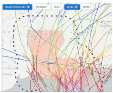
Historical Hurricane Tracks
(1851-present) National Oceanic and Atmospheric AdministrationThis interactive tool allows users to explore past hurricanes. It provides detailed information on over 200 storms for Louisiana alone. It allows users to view information on the category, pressure, wind speed, and track and links to the official National Hurricane Center report on the tropical cyclone.
1. Type in location, year, or storm of interest (i.e., Louisiana) 2. A map will appear with the tropical storm tracks that match your search. 3. At the top left of the map, filter by category, sea level pressure, year, area, month, or ENSO cycle to narrow down storms. 4. Click on the storm track on the map or the event on the left menu to view detailed information on the event. 5. Click the PDF icon in the top right of the information box to view the official report on the storm (if available) or the “i” icon for more details.
Gulf Tree
(Time frame varies by product) Northern Gulf of Mexico Sentinel Site Cooperative, Gulf of Mexico Climate Resilience Community of Practice, & Gulf of Mexico Alliance Resilience TeamThis decision support site guides users to the storm surge tools and resources they need along the Gulf Coast through several filters of information, including how much time and effort they are willing to spend on the tool.
1. Choose a Filtered Search to look through all filter categories on one page or choose Guide My Search to walk through questions step by step to achieve what you’re looking for. If you chose the Filtered Search, first choose the Geographic Scope. Click the Louisiana drop-down menu and choose Shoreline to select all coastal parishes or choose specific one(s). 2b. Under Tool Function, select what you’d like to use storm surge information for. You can leave this blank if you’re unsure which to choose. 2c. Under Cost, choose Free. 2d. Under Level of Effort, choose from low, moderate, or high (will determine how advanced the tool is). 2e. Under Climate Change Topics, select the drop-down for Flooding, then check the box for Storm Surge. Explore other drop-down menus in this section to add more filters for additional topics. 2f. Click View Tool Matches on the top right to go to the results page. Click any of the tools or resources to go to that site.
3a. If you chose Guide My Search, Gulf Tree will walk you through the same filters by asking 6 questions. For step 1 (Tool Function), check the box for why you need a storm surge tool, then click Submit. If you’re not sure which option to use, you can Skip this step. 3b. Step 2 (Topic Area) includes a filter for what aspect of the topic you’re interested in. Click the drop-down menu for Flooding and check the box for Storm Surge. Then, click Submit. 3c. On Step 3 (Location), click the Louisiana drop-down menu, then choose Shoreline to select all coastal parishes or choose specific one(s). Then, click Submit. 3d. For Step 4 (Level of Effort), choose how much effort you’d like to put into the tool, which will determine how advanced the tool is. Then, click Submit. 3e. For Step 5 (Tool Cost), choose Free, then click Submit. 3f. Click Leave Guided Search and View Matches to go to the results page or go back to a previous page on the left menu to change your selected options. Click any of the tools or resources to go to that site. 6. To create a new search, click Reset All Filters at the top right of the results page.
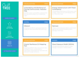
Climate Change Trends
While uncertainty exists in climate models, current research projects the overall frequency of hurricanes to decrease, but their intensity may increase (Easterling et al. 2017). Water temperatures in the Gulf have increased, fueling hurricanes and causing harm to coastal ecosystems (Carter et al. 2018). Furthermore, rapidly intensifying hurricanes have occurred more frequently in recent years and are projected to increase in the future, although this is an ongoing area of research with uncertainty (Bhatia et al. 2022; Emanuel 2017). This phenomenon and a growing population along the coast create an increased risk and exposure to this threat. Future sea level rise also exacerbates storm surge levels, allowing water to reach further inland than in the past. A 1-meter rise in sea level can cause a doubling of storm surge risk (Nielsen-Gammon et al. 2021). Read more about future hurricanes, tropical storms, and storm surge in Climate Change Science and Projection Resources.
Lightning
Data Limitations
Historically, most lightning data have been proprietary, therefore, climatological records of the hazard are limited. However, a new NOAA satellite became operational in late 2017 and contains a significant technological advancement called the Geostationary Lightning Mapper (GLM). The GLM can detect the presence of total lightning including in-cloud, cloud-to-cloud, and cloud-to-ground. While this advancement will not provide historical lightning data, it will add to the climatological record as time goes on.
Definition and Description
A visible electrical discharge produced by a thunderstorm. The discharge may occur within or between clouds, between the cloud and air, between a cloud and the ground or between the ground and a cloud (NWS 2009).
Lightning forms from charge separation within thunderstorms, usually cumulonimbus clouds. Lightning is essentially a large spark of static electricity, similar to touching a doorknob on a dry day (although much more powerful). Most lightning forms from streamers that work their way down from the charge centers of clouds toward the ground. When it gets close to the ground, a return stroke is initiated, which we see as a flash of light. Thunder is created by a shock wave from rapid heating of the air to 18,000 degrees – hotter than the surface of the sun.
Lightning is capable of striking as far as 10 miles away from a storm. Distance can be estimated by counting the seconds between the flash and the sound of thunder. It takes 5 seconds for the shockwave to travel one mile. Lightning severity is not rated, although new detection systems allow accurate identification of lightning strikes allowing analysis of lightning frequency.
Historical Data
Lightning Climatology Tool
(1995-2019) NOAA/National Weather Service Storm Prediction CenterThis tool provides a daily and hourly lightning climatology and shows the probability of at least one cloud-to-ground (CG) lightning strike occurring each day of the year or each 1-hour or 4-hour period throughout the day. It can be used to assess the time of day and time of year with the highest probability of CG lightning. 1. Zoom in to your area of interest on the map. 2. The default map shows the daily (24-Hour) lightning probability on January 1, as indicated in the map title. To select a 1-Hour or 4-Hour climatology, hover your mouse over the Lightning tab at the top of the page and select 1-Hour or 4-Hour. To view other days or hours, move the horizontal scroll bar under the map. Note: the map title and scroll bar show hours in UTC format. 3. Click your area of interest on the map to view the probability of CG lightning occurring on that day or hour for that area. 4. Click the Time Series button within the pop-up box to view a graph of average CG lightning probability for your selected daily/hourly option. You can use this graph to quickly assess the time of year/day that location experiences the most CG lightning. Hover your mouse over the graph for details. Note for hourly options: the box shows local time, unlike the map title. The 4-hour graph will show the probability of at least one CG lightning strike occurring within a 4-hour window (e.g., the value for 12pm will show the probability of lightning occurring between 8am-12pm). 5. If you selected the 1-hour or 4-hour option, click the Heat Map button within the pop-up box to view a graph of 1-hour or 4-hour lightning climatology by both day of year (horizontal axis) and time of day (vertical axis). Darker colors represent a higher probability. Hover your mouse over the graph to assess what time of year and day that lightning is more likely to occur in your area.
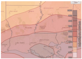
Annual and Monthly Distributions of Cloud-to-Ground Lightning
(1995-2019)NOAA National Severe Storms Laboratory / Cooperative Institute for Mesoscale Meteorological StudiesThese static maps show the cloud to ground lightning density (strikes per km2) in Louisiana, averaged over the years 1995-2019. There are five maps on the document that display annual and seasonal (winter, spring, summer, and fall) densities. 1. Click on the link below. 2. Annual and seasonal maps are displayed with a brief description.
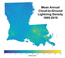
Vaisala Annual Lightning Report and Global Lightning Density Map
(Varies by year) VaisalaThis Annual Lightning Report page provides annual reports since 2017 that contain maps of average cloudto-ground flash density and total lightning density for the previous 5-10 years in the U.S. The reports also offer high-resolution local- and parish-level maps and information. Other features of this site are an archive of past annual reports, supplemental statistics, and a global lightning density map with parish-level data.
1. Click on the link to access Vaisala’s Annual Lightning Report page. 2. Scroll down to the Resources section and click the most recent Annual Lightning Report. 3. Scroll down the document to view various maps, such as total lightning density and cloud-to-ground flash density maps in high resolution and aggregated by parish. 4. To view average lightning density for each parish, click the Global lightning density map from the Annual Lightning Report homepage below Resources. 5. Zoom in until you see parish-level data. 6. Hover your mouse over a parish to view the total lightning density per km2/year from 2016-2021. Note: this map may be updated yearly, so check the About section on the left to confirm the time period.
Climate Change Trends
Studies have shown an increase in lightning associated with severe storms (Schultz et al. 2011). Climate models project an increase in the types of weather conditions that favor severe thunderstorms (Kossin et al. 2017), therefore, lightning occurrences could increase. Confidence in the projections is currently low, however, due to the isolated and sporadic nature of lightning events and limited comprehensive datasets, making it difficult to track long-term trends (Wuebbles et al. 2017a).
Sea Level Rise
Data Limitations
The tide-gauge network is sparse, so there is a lack of tide data for many coastal communities and inconsistent periods of records for locations that do have gauges. Satellite measurements provide better coverage, but do not provide a long-term record. Therefore, it can be difficult to obtain local long-term trends. Sea level rise projections include uncertainties in the rate of ice sheet melting in Greenland and Antarctica, changes in the Gulf Stream and land motion, and future greenhouse gas emissions.
Definition and Description
Long-term increases in mean sea level, the arithmetic mean of hourly heights observed over some specified period (AMS 2020).
Sea level rise occurs due to a combination of melting glaciers and ice caps and from thermal expansion. A vast amount of water is stored in ice caps, primarily in Antarctica and Greenland, which accounts for 50 times the volume of water compared to all the available surface water in lakes, rivers, and seasonal ice and snow. As global temperatures warm, ice sheets are melted which add their water to the surface level of the oceans.
As the temperature of water warms, molecules push farther apart, known as thermal expansion. Thermal expansion creates as great a contribution to sea level rise as does melting ice sheets.
Over the past 100 years, global sea level has risen, on average, 4-8 inches. Half of this is due to thermal expansion and the other half from glacial melt. Sea level is projected to increase by at least 3-4 feet by the end of the 21st century. This is enough to move the shoreline inward by 1,000 feet on average and to inundate 7,800 square miles of North America.
Historical Data
Relative Sea Level Trends
(Period of record varies by gauge; up to ~150+ years)NOAA Center for Operational Oceanographic Products and Services (CO-OPS)This tool uses historical tide gauge data to provide local relative sea level (RSL) trends, which takes into account sea level rise and local vertical land motion. It also provides a time lapse of satellite imagery via Google Earth to visualize the changing coast over time.
1. Click Gulf Coast above the map or pan and zoom to the Texas coast on the map. 2. Click a gauge location on the map, represented by an arrow. Note: use the legend under the map for a quick look at the trend for this location. Warmer colors and arrows pointing up represent an increasing trend. 3. A summary of the RSL trend is shown in the pop-up box. 4. Click Linear Trend in the box to view a graph of the RSL trend over time at this location. The summary of the trend information is included below the graph. You can export the data or save the image using the buttons under the graph. 5. To view a time lapse of satellite imagery via Google Maps, click Landsat Imagery from the pop-up box in Step 3. 6. This default image is zoomed into the selected gauge location. You can zoom in and out by using the +/- buttons on the top right of the page. You can also pause the time lapse and view individual years on the bottom of the page.
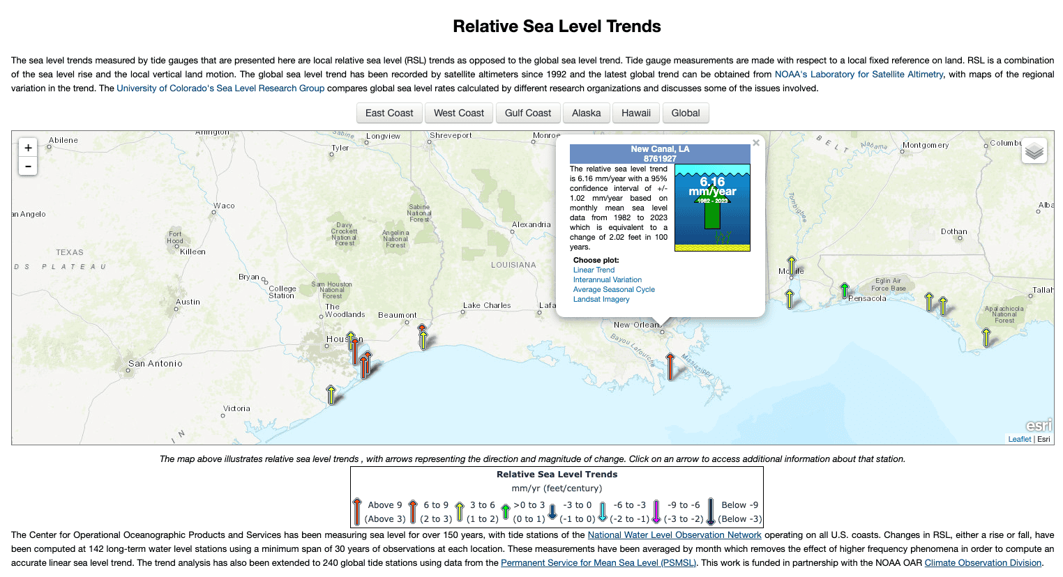
Gulf Tree
(Time frame varies by product)Northern Gulf of Mexico Sentinel Site Cooperative, Gulf of Mexico Climate Resilience Community of Practice, & Gulf of Mexico Alliance Resilience TeamThis decision support site guides users to the sea level rise tools and resources they need along the Gulf Coast through several filters of information, including how much time and effort they are willing to spend on the tool.
1. Choose a Filtered Search to look through all filter categories on one page or choose Guide My Search to walk through questions step by step to achieve what you’re looking for. If you chose the Filtered Search, first navigate to Geographic Scope. Click the Louisiana drop-down menu and choose Shoreline to select all coastal parishes or choose specific one(s). 2b. Under Tool Function, select what you’d like to use sea level rise information for. You can leave this blank if you’re unsure which to choose. 2c. Under Cost, choose Free. 2d. Under Level of Effort, choose from low, moderate, or high (will determine how advanced the tool is). 2e. Under Climate Change Themes, select the box for Sea Level Rise. 2f. Under Climate Change Topics, select the drop-down for Flooding, then check the box for Sea Level Rise if you are interested in flooding associated with sea level rise. Explore other drop-down menus in this section to add more filters for additional topics. 2g. Click View Tool Matches on the top right to go to the results page. Click any of the tools or resources to go to that site.
3a. If you chose Guide My Search, Gulf Tree will walk you through the same filters by asking 6 questions. For step 1 (Tool Function), check the box for why you need a sea level rise tool, then click Submit. If you’re not sure which option to use, you can Skip this step. 3b. Step 2 (Topic Area) includes a filter for what aspect of the topic you’re interested in. Click the drop-down menu for Flooding and check the box for Sea Level Rise if you are interested in flooding associated with sea level rise. Then, click Submit. 3c. On Step 3 (Location), click the Louisiana drop-down menu, then choose Shoreline to select all coastal parishes or choose specific one(s). Then, click Submit. 3d. For Step 4 (Level of Effort), choose how much effort you’d like to put into the tool, which will determine how advanced the tool is. Then, click Submit. 3e. For Step 5 (Tool Cost), choose Free, then click Submit. 3f. Click Leave Guided Search and View Matches to go to the results page or go back to a previous page on the left menu to change your selected options. Click any of the tools or resources to go to that site. 6. To create a new search, click Reset All Filters at the top right of the results page.
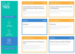
Climate Change Trends
Sea level on the Gulf Coast is projected to increase by 14-18 inches by 2050, which is more than the rise measured over the last 100 years (Sweet et al. 2022). Based on current emissions, 2 feet of sea level rise is expected along the U.S. coast between 2020-2100 (Sweet et al. 2022). Without reducing emissions, 3.5-7 feet of sea level rise may occur by 2100. The western Gulf Coast has the highest rates of sea level rise because of the high rates of subsidence, which has caused a loss of nearly 2,000 square miles of land since the 1930s (Frankson et al. 2022). This subsidence has caused Louisiana’s rate of sea level rise to be four times higher than the average global rate (Frankson et al. 2022). Sea level rise exacerbates coastal flooding and increases saltwater intrusion, which contaminates fresh groundwater supplies. Researchers are actively working to improve ice sheet dynamics and sea level rise modeling to further understand and enhance future projections. Read more about future sea level rise in Climate Change Science and Projection Resources.
Coastal Change Hazards Portal
(Shoreline Change Forecasts: 50-100 years) U.S. Geological SurveyAccess this tool to view the Coastal Vulnerability Index and forecasted shoreline changes from sea level rise.
1. To view projections of vulnerability to sea level rise, zoom in to the area of interest 2. Select Sea-Level Rise from the righthand menu. 3. Select Coastal Vulnerability Index then the option for the Gulf of Mexico to view an area’s vulnerability to sea level rise. Or select Shoreline Change Forecasts → Probabilities of Shoreline Change for Contiguous U.S. then select one of the retreat/advance options (e.g., Probability of high shoreline retreat) to view the probability of future shoreline change over the next 50-100 years. Click the colored line on the map or refer to the legend to determine the risk value or long-term change at that location.
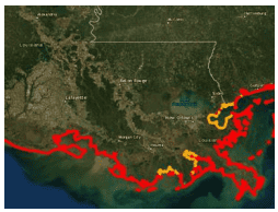
Sea Level Rise Viewer
(SLR: Present-2100, Local Scenarios: 2000-2100)National Oceanic and Atmospheric AdministrationThis mapping tool visualizes the impacts of sea level rise and includes local photo simulations of what sea level rise may look like at select locations. The tool allows users to choose different water levels to view sea level rise projections, overlay community vulnerability, and view local scenarios by year.
Click Get Started. 2. Zoom into the area of interest. The default map is the current water level, where darker blues are greater water depths. 3. Adjust the vertical slider on the left to project different water levels. 4. To view a photo with simulated water levels, click an icon on the map (may need to zoom in). 5. Click Local Scenarios on the lefthand menu to view relative sea level rise by year and for different scenarios. Click any scenario icon on the map to change locations. 6. View by Scenario tab: Select a local scenario by sliding the scenario marker on the right to view the amount of relative sea level rise associated with that scenario in 20-year increments displayed on the left. View by Year tab: Select a year by sliding the year marker on the right to view the amount of relative sea level rise associated with that year for each of the local sea level rise scenarios on the left. 6. Click Vulnerability on the lefthand menu to overlay social and economic data to see the potential impact to sea level rise. Note: Access the legend by clicking the middle icon on the top right of the screen.
Severe Thunderstorm Winds
Data Limitations
Population and temporal biases (i.e., a greater number of reports in recent decades), a limited number of weather stations that record wind speed, and the highly localized nature of severe thunderstorm winds, mean that data are not of sufficient quality to robustly determine whether there have been trends over a long period of time (e.g., 100+ years).
Definition and Description
High winds are defined as sustained non-convective wind speeds of 40 mph or greater lasting for 1 hour or longer, or gusts of 58 mph or greater for any duration.
Severe thunderstorm winds are winds of 58 mph or greater when convection (i.e., thunderstorm) is present.
High winds can occur with thunderstorms, but also with frontal passages and gradients between areas of high and low pressure. There are several types of wind events.
- Straight-line winds are thunderstorm winds that do not have rotation and are different from tornadic winds.
- Downdraft winds can also be damaging and are a small column of air that rapidly sinks toward the ground.
- Downbursts describe wind events that are caused by a strong downdraft within a thunderstorm.
- Microbursts are small concentrated downbursts that produce an outward burst of strong winds at or near the surface.
Wind speeds and the effects can be measured by the Beaufort Wind Scale (NWS 2024), which ranges from 0 (calm winds) to 12 (hurricane-force winds).
Historical Data
Severe T-Storm Wind Days Per Year
(1986-2015)NOAA/National Weather Service Storm Prediction CenterThis map shows you the average number of days per year in which severe thunderstorm wind reports were received in your area. The map gives you a sense of the approximate number of days each year that you can expect to see severe thunderstorm winds (57 mph or greater) in your area.
1. Select any of the three wind climatology maps to view a larger image: Greater Than 50-Knots & Less Than 64-Knots, Greater Than 64-Knots, or All Wind Greater Than 50-Knots. Note: 50 knots is equal to 57 mph; 64 knots is equal to 73 mph.

Severe T-Storm Wind Reports
Wind: (1955-present) Southern Regional Climate CenterThis interactive tool shows you the historical record for individual severe thunderstorm wind reports (gust of 57 mph or greater) in your area. It can be used to determine severe thunderstorm wind events that have impacted your area or nearby.
1. On the left side of the screen, click on Search within Radius. 2. Choose the diameter of the area of which you want to investigate (25 or 50 miles). 3. Pan, zoom, and then click on the map area of interest. 4. Select Wind (de-select other hazards). 5. Reports are displayed on the map and in two tables below the map. 6. Map: Mouse over individual storm reports for details. 7. Tables: There are two tables, Recent Storm Data and Historical Storm Data. Click on the column header to sort by column of interest. For example, to view the dates on which the highest wind occurred, click on the Scale column headers to sort by the highest wind value.
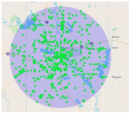
Severe T-Storm Watch Climatology Map
(2004-2023) NOAA/National Weather Service Storm Prediction CenterThis map shows a 20-year climatology of severe thunderstorm watches. From this map, you can get a sense of the approximate number of days each year you can expect to have a severe thunderstorm watch issued for your parish.
1. Under the Storm Prediction Center WCM Page banner near the top of the page, click on the Watch Frequency Maps link. 2. Scroll down a bit until you see 20y SPC Watch Climatology. 3. Click on the Average number of severe thunderstorm watches per year image to view it in larger form. Note: this WCM page contains a lot of other statistics about the hail, severe thunderstorm, and tornado products that come out of the NWS Storm Prediction Center if you are interested in digging deeper into the data.
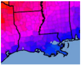
Climate Change Trends
Damaging winds in Louisiana are associated with both tropical storms and thunderstorms. Louisiana has the second-highest frequency of thunderstorms per year, on average, in the contiguous U.S. (Frankson et al. 2022). More favorable environments for severe thunderstorms are expected, especially during the peak storm season (March-May), so associated increases in severe wind occurrences are projected. It is not known, however, whether the favorable environments will reach their potential of producing damaging winds (Kossin et al. 2017). Historically, severe thunderstorm winds have occurred more often in northern Louisiana.
Tornado
Data Limitations
Tornado reports prior to the 1980s were compiled from written records. Consequently, many tornadoes were unreported or multiple tornadoes may have been listed as a single event. Tornado tracking is unique as occurrences are recorded either by damage assessments or visual accounts (Kossin et al. 2017). Advanced radar technology, increases in rural populations, usage of video and social media, emphasis on documentation, and improvements in communication have resulted in an increase in the number of reports, especially among weaker (EF0-EF1) tornadoes. Due to these known systematic biases, use caution when assessing long-term trends based solely on the number of reports.
Definition and Description
A violently rotating column of air, usually pendant to a cumulonimbus, with circulation reaching the ground. (NWS 2009)
Tornadoes generally form from severe thunderstorms, particularly supercell thunderstorms – those that are isolated with unimpeded inflow of moisture and enhanced by wind shear. Tornadoes may also form along squall lines or in bands of storms associated with hurricanes. Tornadoes require moist air, instability (warm air rising), a source of lift such as a front, dryline, or heating, and wind shear (change in wind direction and speed with height).
Tornadoes can occur at any time of the year and at any time of the day. Arkansas experiences an uptick in tornadoes in the spring, but they also see tornadoes in the fall and winter as the jet stream moves toward the south.
Tornado intensity is rated by the damage they produce, on a scale from EF0 (weak) to EF5 (violent). Strong (EF2-EF3) and Violent (EF4-EF5) tornadoes account for only about one-third of all tornadoes, but 97% of fatalities and the vast majority of economic impacts. Tornadoes along squall lines and hurricane bands are more likely to be weak, although widespread severe straight-line winds may accompany these types of storms.
Historical Data
Tornado Tracks Tool
(1950-2023)Midwestern Regional Climate CenterThis is an interactive tool that shows historical tornado track details by track location or parish. Consider nearby storm tracks, even if they did not hit your location, because small changes in storm motion can bring a tornado into your town.
1. Select the area of interest either by zooming or entering a location into the search box. 2. Use the panel on the left side of the screen to select variables of interest. Options include by Magnitude, Year Range, Month, and Casualties. 3. To view information about a tornado track, select Track in the left panel and hover your mouse over the track on the map. 4. To view an image of all tornado tracks in a parish, click County from the left panel and click a parish on the map.

Tornado Risk Assessment
(1950-2019) NOAA/National Weather Service Storm Prediction CenterThis site displays a series of graphs that shows tornado occurrences and statistics based on a given point. Statistics include F/EF scale frequency and probabilities of strikes occurring by month and time of day.
1. Click on the black bar at the top of the page (bar includes location, radius, and time period information) and provide the zip code of interest. A suggested radius input is 40 km (~25 mi). 2. Click Run. 3. Details about tornadoes that have occurred within the selected area are displayed on the page.
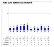
Tornado Days Maps
(1986-2015)NOAA/National Weather Service Storm Prediction CenterThese static maps show the average number of tornado days per year for all magnitudes (separate maps show EF1+, EF2+ and EF4+ days) within 25 miles of any point from 1986-2015. Tornado frequencies at a given location can be compared to nearby and regional locations.
1. Click on any of the four Tornado Climatology maps to view a larger image: All Tornado Days, EF1+, EF2+, or EF4+ Tornado Days.
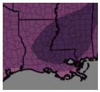
Tornado Watch Climatology Map
(2004-2023)NOAA/National Weather Service Storm Prediction CenterThis map shows you a 20-year climatology of tornado watches. From this map, you can get a sense of the approximate number of days each year you can expect to have a tornado watch issued for your parish.
1. Under the Storm Prediction Center WCM Page banner near the top of the page, click on the Watch Frequency Maps link. 2. Scroll down a bit until you see 20y SPC Watch Climatology. 3. Click on Average number of tornado watches per year image to view it in larger form. Note: This WCM page contains a lot of other statistics about the hail, severe thunderstorm, and tornado products that come out of the NWS Storm Prediction Center if you are interested in digging deeper into data.
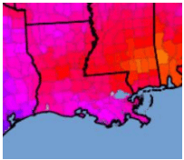
Storm Events Database
Tornado: (1950-present)This interactive tool shows you the historical record for individual tornado reports by county. It can be used to determine tornadoes that have impacted your area or close to your area.
1. On the bottom left, under Select State or Area, choose Louisiana → then Search 2. From top to bottom, select a specific Begin and End Date, as well as County of interest. 3. Under Event Type(s), select Tornado. 4. Under Advanced Search and Filter Options → Tornado Filter, select tornado rating of interest or leave as All Tornadoes. 5. Press Search. Summary results are presented in a table. 6. Click each hyperlinked location name to view more information, read the storm narrative, and view the storm track. Note: This tool can be used to analyze a variety of additional hazards with various time periods, and tornado data goes as far back as 1950. Property and crop damage estimates are available in the table, but there are many limitations to this data.
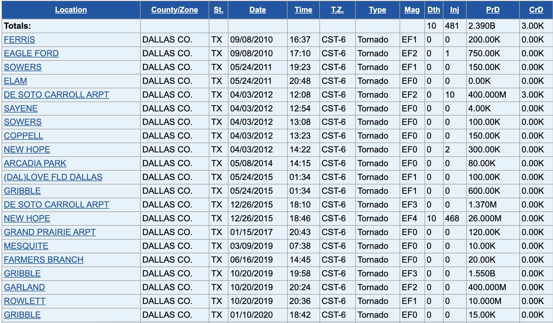
Climate Change Trends
Over the past 40 years, there have been an increase in the frequency of days with a large number of tornadoes (i.e., tornado outbreaks) in the U.S. However, there has also been a decrease in the frequency of days with tornadoes (Kossin et al. 2017), meaning that more tornadoes are occurring on tornado outbreak days than on isolated days. Because the severe thunderstorms that produce tornadoes (e.g., supercell thunderstorms) occur on such a small scale, climate models have difficulty resolving future trends. However, if one looks at the larger scale “ingredients” needed for tornadic storms, there will likely be more days where such storms are viable (Nielsen-Gammon et al. 2021). In Louisiana, tornadoes may also occur within hurricanes and tropical storms, and tornadoes have historically occurred more frequently in eastern Louisiana.
Wildfire
Data Limitations
A systematic, national collection of wildfire reports did not begin until the early 1990s. Many analyses are based on only a few years of data, which may not capture multi-year variability or trends. Further, fires accounted for by local jurisdictions may not always translate into national databases.
Definition and Description
Any free burning uncontainable wildland fire not prescribed for the area which consumes the natural fuels and spreads in response to its environment (NWS 2009).
Wildfires occur when weather conditions meet with sufficient fuel and an ignition source. Weather conditions include warm temperatures, low humidity, strong winds, and a period without precipitation allowing fuels to dry. Fuels are vegetation ranging from fine fuels such as grass and pine needles to large woody materials such as trees, dead and decaying logs, and organic material in the soil. Large woody materials are difficult to ignite; the presence of fine fuels allows fire to get started and become intense enough to ignite larger materials. Ignition sources may be natural such as lightning or human-caused such as sparks from equipment, power transformers, a chain dragging behind a vehicle, or heat sources such as discarded cigarettes.
Usually wildfires occur when the state experiences a drought, but they can still happen at any time. Fires are a common occurrence during a drought when dried vegetation provides fine fuels and warm, windy, dry days provide weather conditions that allow ignition and spread. Summer has higher temperatures that can allow fires to become very intense, but there is typically less wind and consequently less spread. Fire spread may be increased on south-facing slopes, which are usually drier and warmer because of exposure to the sun, windy locations such as canyons, and along steep slopes. Very intense fires may become “crown fires” if they burn to the tops of trees, allowing embers to spread farther and create spot fires. Crown fires are almost impossible to extinguish without cooler, wetter weather conditions.
Fire danger is measured on a Burning Index scale, ranging from 0 to 110+. Values below 20 are considered low fire potential, 40-80 is high, and 110 or higher is extreme. The burning index combines potential energy release (fire intensity), flame length, and rate of spread. The National Weather Service issues Red Flag Warnings when weather conditions are favorable for ignition and spread of wildfires. Another popular index is the Keetch-Byrum Drought Index (KBDI) that considers weather and vegetation conditions. The scale ranges from 0 to 800; values below 200 indicate high fuel moisture making ignition unlikely; values above 600 are indicative of intense wildfire conditions with any that develop capable of downwind spotting (starting new fires).
Historical Data
Wildfire Risk to Communities
(Varies by data layer; fire occurrence: 1992-2020, fuelscape: 2020)USDA Forest ServiceThis tool provides information and resources for communities to understand, explore, and reduce wildfire risk. Mitigation resources and programs for action are provided in the Incentive and Action Programs for Hazard Risk Reduction menu item, but this segment of the tool allows users to explore risk for a community, tribal area, county, or state. This tool provides several charts and maps about wildfire risk and compares the risk of your selected area to other jurisdictional levels.
1. In the search bar, enter your desired community, tribal area, county, or state. 2. On the results page, you’ll see a summary statement comparing your selected area’s wildfire risk to the rest of the nation. Below this is a summary of the risk to homes, wildfire likelihood, risk reduction zone, and vulnerable populations, with a risk of low to high. 3. Select one of these risk categories to view more information and access an interactive map. 4. The resulting page includes a summary statement, interactive map, descriptive information about that risk, and action information. 5. The Risk to Homes and Wildfire Likelihood options include an interactive graph of percentiles that compares your selected area to others. The default geographic comparison is Nation but you can select a different option (e.g., county or state) from the Compare to drop-down menu at the top of the page. Hover over the points on the graph to explore the information (red points represent higher risk or likelihood). Switch to other risk pages by using the tabs on the top of the page.
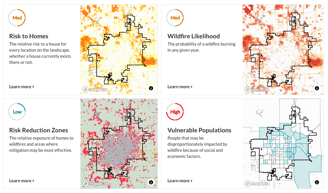
National Interagency Fire Occurrence
(1992-2018) K. C. Short/ U.S. Department of Agriculture, Forest ServiceThis interactive tool shows the location of reported fire occurrences between 1992-2018 in and near a parish or city. Individual years can be viewed to determine relative risk. Many fires in urban areas are not reported to the U.S. Forest Service database, however, so it may under-represent fire risk in urban areas. Note: There is a learning curve associated with this tool and it is helpful to use a larger computer screen because of the amount of data shown.
1. Click on the Map View link below. 2. Next to View In, click ArcGIS Online map viewer. A new internet browser tab will open. 3. On the left side of the screen, under Contents, expand EDW FireOccurrence5thEdition 01 on the top by clicking the arrow to the left of the name. 4. Select year(s) of interest or All Years (last in the list). 5. Zoom in on the map if data are not shown. 6. To view Louisiana fires only, hover your mouse over the year of choice in the left-hand menu and click on the filter icon (fourth from the left). 7. Select STATE in the left drop-down menu → In far-right box enter LA → Click APPLY FILTER. 8. A table containing the details of each fire can be viewed by clicking the table icon (two icons left of the filter icon when you hover over the left-hand menu). 9. The map symbols represent varying causes of wildfire occurrences. To view the legend, click on the legend button at the top right of the left-hand menu. 10. To view data on an individual fire, open the table from Step 8 and then click on the fire symbol of interest on the map. In the top right-hand corner of the table, click on the three horizontally lined tab and select Show Selected Records. Details of the selected fire will be displayed in the table. 11. Refer to the paper linked below for table column definitions. Note: Additional filters can be applied by clicking on the filter icon again and choosing desired selections (e.g., the column STAT_CAUSE_DESCR describes the cause of the fire).
Original Paper (open access): https://www.fs.usda.gov/rm/pubs_other/rmrs_2014_short_k001.pdf
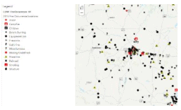
Southern Wildfire Risk Explorer
(Wildfire Ignition Density: 1997-2002; other layers based on various risk assessments)Southern Group of State ForestersThis interactive tool can be used to identify areas within and/or near a city that are at the greatest risk of wildfire. It is especially useful for identifying risk areas in the wildland-urban interface and to help prioritize areas where tactical analyses, community interaction, or mitigation treatments might be necessary to reduce risk. Note: There is a learning curve associated with this tool. Basic Viewer is accessible to anyone. Advanced Viewer is also free but requires account request.
1. Scroll down to the Tools section and click Southern Wildfire Risk Explorer. 2. On the next page, select Basic or Advanced Viewer. The following instructions are for the Basic option. 3. Pan and zoom-in on the map to area of interest. 4. Click on Map Themes in the upper left-hand corner. 5. Under the Wildfire Risk section on the left side of the screen, select the layer you want to view. Details about each layer (including legend information) can be found by hovering over the circular “i” icon. 6. To compare layers, such as WUI Response Index and Community Protection Zones, click on the second icon (divider) under the search bar at the top right of the page. You can choose two selections from the drop-down menus. Note: Data are displayed at a very fine (25-meter) resolution, so you may need to greatly zoom in to view more details on the map. The Advanced version of this tool provides many more features, including the ability to upload your own shapefiles, download the map and associated GIS data for your area, generate a risk summary report for your area, and download an editable summary report to be used for Community Wildfire Protection Plan (CWPP) development.
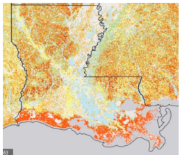
Wildland-Urban Interface
(1990, 2000, 2010, 2020) University of Wisconsin-Madison SILVIS LabThis interactive tool shows WUI (Wildland-Urban Interface) changes between 1990, 2000, 2010, and 2020 for locations of interest. It shows the effects of housing growth on the environment and which areas may need more local land management related to WUI issues.
1. Zoom in to the desired location on the map. 2. On the left side of the screen, select year, base map, and layer opacity of interest. Note: Louisiana-specific data and map files (down to the parish level) are available by scrolling down the page.
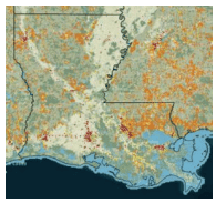
Wind Rose Plots
(Period of record varies by station; up to ~85 years) Iowa Environmental Mesonet, Iowa State UniversityView common and prominent wind speeds and directions for your area. Plots can be viewed by monthly average and by the long-term yearly average. This tool can be used to view the wind climatology and the predominant direction in which air pollutants flow. It may also be useful for understanding how wildfire events may evolve in a community.
1. In the Select By Network section, choose Louisiana ASOS then click Switch Network. 2. Select station of interest, either from the list or map, then click Select Station. 3. You will be brought to a new page. Near the top of the page, click on the Wind Roses tab. 4. The yearly climatology plot is displayed at the top of the page, and monthly climatology plots are displayed below that. Click View Raw Data on any plot to view more details.
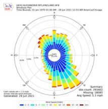
Climate Change Trends
From 2007-2016, nearly 15,000 acres of forest burned from wildfires in Louisiana on average each year (LDAF 2022). Louisiana includes protected forests in the north and flash fuel areas in the southeast and southwest, where historical wildfire probability is higher and projected to worsen by 2050 (LDAF 2022; Mostafiz et al. 2022). Wildfires may become more frequent in Louisiana with increased dryness of vegetation from increased temperatures and decreased summertime rainfall in the future (Hayhoe et al. 2018). More urban development near forests can also lead to a decrease in prescribed burns to manage wildfire (Carter et al. 2018). Wildfires in Louisiana are dependent upon current weather conditions, seasonal climate patterns, vegetation conditions, and an available source for ignition (such as a spark, flame, or intentional ignition). Given this complex relationship, the future trend for wildfire is also complex. Read more about future wildfire risk in Climate Change Science and Projection Resources.
Historical and Projected Wildfire Probability and Property Loss
(Historical: 1992-2015, Projected: 2050)Mostafiz et al. 2022This article includes maps of historical (1992-2015) and projected (2050) annual probability of wildfire occurrence and annual average property loss from wildfire in Louisiana. Parish-level information is also included in the appendices.
1. Click the link below to access the paper. 2. Scroll to Section 6. Results. Historical (1992-2015) and projected (2050) annual probability of wildfire occurrence (%) is shown in Figure 1. Figure 1a also shows the 12 parishes with the highest wildfire frequency from 1992-2015. 3. Historical (1992-2015) and projected (2050) annual average property loss is shown in Figs. 3-6. The left map for each figure represents the historical estimate and right map shows the projected future estimate. Read Section 6 to learn more context about the figures. 4. Scroll to Appendices A-D for parish-level information related to the figures. Note: there are many limitations to property loss estimates, so the values in Appendix D should be used with caution. However, you may use this table to identify if a parish is projected to have an increasing/decreasing trend in property loss by 2050.
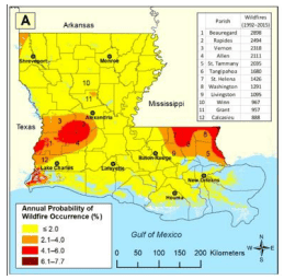
Winter Storm (Ice, Sleet, Snow)
Data Limitations
Long term records are limited because of the difficulty in observing ice storms/freezing rain (e.g., rain, freezing rain, and snow can occur at a single station during a single event).
Definition and Description
A winter storm is a winter weather event that produces impactful accumulations of freezing rain (ice), sleet, and/or snow (NWS 2018).
Winter storms may include heavy snowfall, blowing and drifting snow, high winds, extreme cold or ice storms. Among the greatest hazards associated with winter storms are traffic accidents. The most extreme instance is a blizzard, which is defined as winds greater than 35 mph, visibility less than ¼ mile, lasting at least 3 hours. New snowfall is not necessary for a blizzard, and blowing snow can similarly obscure visibility.
Winter storms are measured by snowfall accumulation or ice thickness. Northern Louisiana has a higher chance of experiencing a winter storm than other areas of the state. Winter storms that occur in Louisiana are usually created by large low-pressure systems moving rapidly across the country. In Louisiana, ice storms and freezing rain are a greater threat than blizzards or heavy snowfall. Access to moisture from the Gulf of Mexico falling over shallow cold air near the surface can produce ice accumulations that can impact power distribution and transportation.
Historical Data
Snowfall Climatology Toolbox
(Period of record varies by station; ~30-100+ years) Midwestern Regional Climate CenterThis interactive tool shows normal (1991-2020) annual and monthly snowfall, average annual number of days with snow totals at certain thresholds, average first and last snow date, and record 1-day snowfall. The map displays normal values while the graph below it shows the variable by year.
1. Position map to area of interest or choose LA in the State Selection drop-down menu on the right. 2. On the top of the screen, select a variable you’re interested in (e.g., Annual Snowfall). Some variables have options on the right side of the screen to select, such as a month to display for monthly snowfall or a snow threshold. 3. For most variables, the map displays the normal/average value for the variable you selected. For Record 1- Day Snowfall, it shows the record value at each point. The legend for the colored points is on the top-right side of the screen. 4. The graph below the map shows more details, such as the values per year instead of an average. Note: The map default shows stations with data from at least 1991-2020. If you’d like to see longer time frames, you can move the slider under the Data Available Since option on the right. When you select a different start year, it will only show stations with available data.
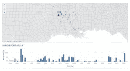
Snowfall Extremes
(Period of record varies by location; up to ~125 years) NOAA National Centers for Environmental InformationThis interactive static map shows the 1-day, 2-day, and 3-day snowfall maximums by parish.
1. Select the day-length of interest on the top right side of the map. 2. Click on the parish of interest for information on the maximum snowfall event on record for your selected time period. 3. A table below the map shows location (by parish and station), date of event, and snowfall total details. Click the top of the right two columns to sort by date or value.
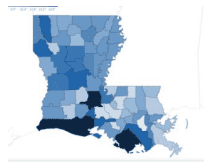
The Frequency of Freezing Rain
(days: 1948-2000; hours: 1932-2001)Midwest Regional Climate CenterThis page includes information about ice storms, including frequency maps of the average annual number of days and hours with freezing rain. Other resources and information, such as preparedness actions, are provided as well.
1. Under the webpage’s heading, click the Frequency tab or scroll down until you reach the section The Frequency of Freezing Rain. 2. View the top map for the average annual number of days with freezing rain from 1948-2000 or the bottom map for the annual average number of hours with freezing rain from 1932-2001. Note: These maps were derived from the journal articles Changnon and Karl (2003) and Changnon (2004). Changnon and Karl (2003) is an open access article and can be found here for further information.
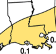
Long-Duration Freezing Rain Events
1979-2016McCray et al. (2019), open accessThis is a figure within a scientific journal article. While the article includes complex scientific information about the meteorological processes behind ice storms, the analysis in Figure 1 shows a climatology of freezing rain and long-duration freezing rain events from 1979-2016 at stations across North America.
1. Scroll down to Figure 1, located in section 3. Regional climatology of long-duration freezing rain. 2. Click View Full Size under Figure 1 to enlarge the image. 3. There are 4 maps, including a) median annual freezing rain hours, b) median annual LD (long-duration) freezing rain events, c) percentage of events that are LD (long-duration), and d) number of freezing rain events lasting at least 18 hours from 1979-2016. 4. Each dot on the map represents a weather station. You can view the station closest to your area or read below for a summary of the state.
Figure summary for Louisiana: In map A, we see that most stations across Louisiana do not typically experience freezing rain each year, with the exemption of northern Louisiana that has observed fewer than 10 hours of freezing rain per year. In addition, map B indicates that stations in Louisiana do not typically experience long-duration freezing rain events (or an event lasting more than 6 hours). When freezing rain events do occur, map C shows that 20-50% of events in Louisiana have a long duration. A station in northeast Louisiana observed 40-50% of events as long-duration, which is disproportional to the lack of hours with freezing rain per year. This same station also observed 2-4 freezing rain events lasting at least 18 hours from 1979-2016, shown in map D. Events of this duration are considered in the 99th percentile, which is a rarity. Other stations across the state observed 2 or fewer events. Overall, this figure shows that much of Louisiana has observed few (if any) hours of freezing rain per year; however, when freezing rain does occur, it can be a long duration. This impacts travel, energy, infrastructure, and health.
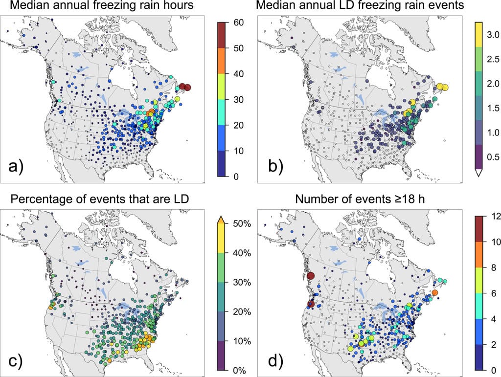
Climate Change Trends
The number of days with maximum temperatures below freezing has been below average since about 1990 in Louisiana, and cold extremes are expected to decrease in the future (Frankson et al. 2022). Models also project that by mid-century there will generally be a northward shift of the rain, sleet, and snow dividing line across the south-central U.S. This shift will add to the complexity of determining precipitation type for winter events (rain, ice, or snow) in Louisiana. However, warmer winters and this shift of precipitation type will likely decrease the number of snowfall and freezing rain events. Read more about future winter storms in Climate Change Science and Projection Resources.
Dam or Levee Failure
Data Limitations
The tools below do not provide dam or levee failure information but rather information on the locations of and pertinent details about dams and levees in Louisiana. The dam inventory is limited to dams with a height of at least 25 feet and which exceed 15 acre-feet in storage, or those with a height of at least six feet and 50 acre-feet of storage unless the dam is classified as high hazard potential. The high hazard potential dam is a dam where failure will probably cause loss of human life regardless of the physical condition of the structure.
Definition and Description
Catastrophic type of failure characterized by the sudden, rapid, and uncontrolled release of impounded water or the likelihood of such an uncontrolled release. It is recognized that there are lesser degrees of failure and that any malfunction or abnormality outside the design assumptions and parameters that adversely affect a dam’s primary function of impounding water is properly considered a failure. These lesser degrees of failure can progressively lead to or heighten the risk of a catastrophic failure. They are, however, normally amenable to corrective action (USSD 2018).
Dams help address the complex challenge of controlling and distributing water. They have been recognized as a key water management practice dating back to early civilizations of the Americas, ancient Egypt, and China. As water is a part of the hydrologic cycle, dams work to conserve water through reservoirs to prohibit flow back to the ocean. With the advancement of civilization and a growing population, water withheld in such reservoirs are an integral part of society and is a necessary source for energy, drinking water, irrigation practices, etc. Dams also protect areas of development and civilization from floods through flood control measures. Dam safety and maintenance standards have increased over time.
Historical Data
National Inventory of Dams by State
(1900-present) U.S. Army Corps of EngineersThis tool provides you with an overview of the dams in Louisiana, including the number by hazard potential, height, owner type, primary type, primary purpose, and completion date.
1. Scroll down until you see a map. On the drop-down menu to the left of the map, select Louisiana. For specific parishes, you can then select a parish within Louisiana from the same menu or click on the map after Louisiana is selected. 2. The map then zooms in to Louisiana and shows all dam locations. A summary of dams in the state are visible above the map. 3. To view dams by hazard potential, click the Layer Controls button on the top left of the map, then click Categorize by and choose Dams by Hazard Potential. The number of dams in each category are shown under the map. Other categories can be mapped as well. 4. Click Browse These Dams above the map to access a list of dams with more information.
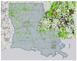
National Inventory of Dams Interactive Report
(1900-present) U.S. Army Corps of EngineersThis report allows you to view the details of individual dams within the state of Louisiana.
1. At the top of the page, click on the Advanced Search tab. 2. On the top left of the page in the Location box, select State for the Geography Type, then type Louisiana in the space below. Click UPDATE RESULTS above this area. 3. Click the DAM DETAILS tab near the top of the page to access a chart of all Louisiana dams and associated information. 4. Choose which columns to display by clicking Columns, then select/de-select the columns as needed. 5. To sort by column, click the arrow to the right of the column header. Note: You can narrow results by selecting additional options on the left of the page (such as Hazard Potential Classification to view high hazard dams). Click UPDATE RESULTS for any changes made to update the list.
National Levee Database
(Levee Inventory: 1882- present) U.S. Army Corps of EngineersThis tool allows you to to explore levees in your area, including location, year constructed, length, number of people and structures at risk should failure occur, property values in the risk area, and more.
1. In the search bar, type Louisiana or a city, parish, address, or levee name. After you type the location or levee name, click the selection from the dropdown menu. 2. The next page shows a map of levees in your selected area and a list of levees on the lefthand side. Click the levee from the list or on the map. If you select the levee from the map, then click it again in the Select a Levee System popup box when it appears. 3. The results page includes information about the levee, including a summary, performance and condition, a map, and the flooding hazard. The Behind the Levee section on the right includes consequence information (e.g., infrastructure, population, property values). Mouse over the squares to see more information.
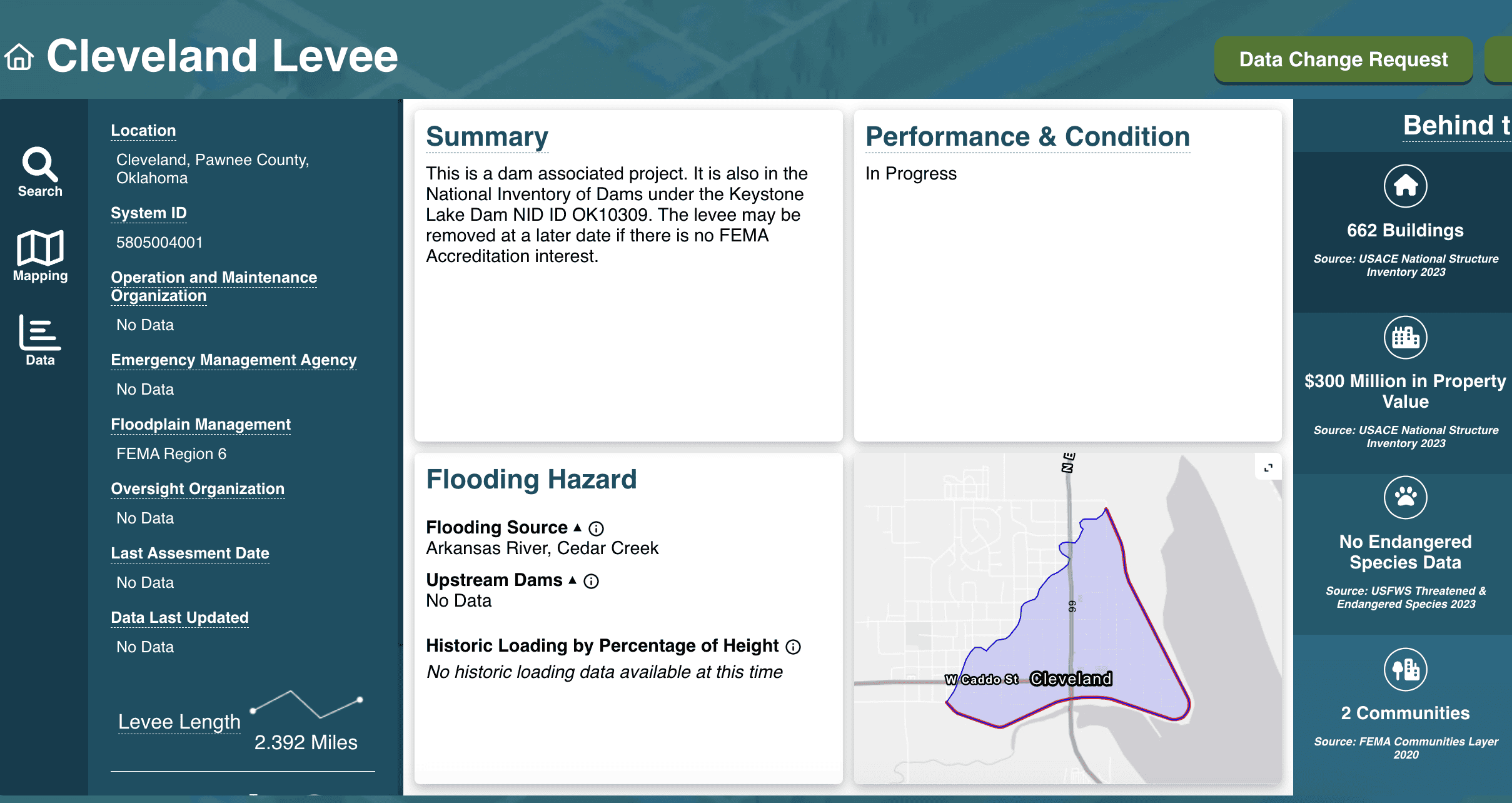
Climate Change Trends
Increases in extreme rainfall (Easterling et al. 2017) may increase the likelihood of dam failure, however, this is highly dependent upon the quality of the structures. The average age of dams and levees in Louisiana is 54 years and 66 years, respectively, and with a 50-year design life, the probability of failure increases with time. Dams and levees that are not well maintained have an increased likelihood of failure. Washed out spillways, deteriorated primary spillway conduits, collapsed riser structures, and slope instability can lead to a dam breach. Furthermore, sediment buildup in reservoirs leads to a decreased capacity, which in turn decreases flood storage. In 2005 during Hurricane Katrina, 50 levees and floodwalls in New Orleans failed (Sills et al. 2008). The U.S. Army Corps of Engineers were awarded billions of dollars in federal funds to build a flood protection system that exceeded the standard 100-year flood event to ensure it would withstand an increased future flood risk (De La Garza 2021). Increased heavy rainfall events and the possibility of stronger tropical storms will heighten the risk of dam failure.
Earthquake
Data Limitations
Globally, scientific understanding of earthquake processes is somewhat limited, and the available history of seismicity is typically too short to establish reliable spatiotemporal patterns of large earthquake occurrences (Stein et al. 2012).
Definition and Description
A sudden slip on a fault, with resulting ground shaking and radiated seismic energy caused by the slip, or by volcanic or magmatic activity, or other sudden stress changes in the earth (USGS 2018).
Earthquakes occur from the sudden release of stress in the Earth’s crust. Stress is built up by the motion of tectonic plates. Stress may also be built up through the injection of fluids. During an earthquake, rocks on either side of a fault line move either horizontally or vertically. This movement creates three types of waves: primary, secondary and rayleigh waves. Primary waves spread outward from the epicenter (source of the fracture) as compression, like a spring. Secondary waves vibrate at right angles to the direction of travel, and these are the most damaging. Rayleigh, or surface, waves move vertically, giving an undulating motion. Earthquake intensity is measured on the Moment Magnitude Scale. Each point represents a 10-fold increase in the wave amplitude and a 32-times increase in energy release.
Most earthquakes that occur in Louisiana are small in magnitude and cause minor damage. An earthquake caused by the New Madrid fault, situated in the Mississippi Valley, could impact Louisiana.
Historical Data
Earthquake Catalog
(Period of record varies by location; up to ~90 years)U.S. Geological SurveyThis tool shows past earthquakes on an interactive map and can be used to show previous occurrences.
1. Under Basic Options, select the Magnitude, Date and Time, and Geographic Region to plot. Choose a Custom date and time with a start date such as “1970-01-01 00:00:00” to view long-term trends. Select a Custom Geographic Region for Louisiana by clicking Custom, then zooming into the pop-up map and drawing a rectangle around Louisiana. 2. Click Search. 3. A map with all earthquakes meeting your chosen criteria are shown and a list of earthquakes are on the left of the page. 4. View the map legend by clicking the key icon on the top right of the map area. To learn more about specific events, click any point on the map or select an event from the list. You can also sort by date or magnitude.
2014 Seismic Hazard Map
U.S. Geological SurveyThis map from 2014 shows the seismic hazards in Louisiana. Louisiana has a low seismicity risk.
Louisiana Earthquake Information Page
U.S. Geological SurveyAdditional information about earthquakes in Louisiana can be found on this page. Click on links of interest.
Climate Change Trends
Louisiana has a low seismicity risk, and the U.S. Geological Survey has only recorded 5 earthquakes since 2000. The earthquakes that have occurred were low in magnitude and caused minimal damage. The New Madrid seismic zone poses a potential threat to Louisiana, which impacted Louisiana and areas in the central and eastern U.S. in the early 1800s (Stevenson and McCulloh 2001). Note: this section of the Simple Planning Tool is titled ‘Climate Change Trends’, but in the case of earthquakes please regard this as future trends.
Poor Air Quality (Dust, Pollutants, Smoke)
Data Limitations
Geographical and spatial gaps exist for air quality data, especially in rural areas. However, areas distant from monitoring stations typically experience consistently good air quality. Also, there is no single air pollutant relevant to every discussion, so there is no single way to express air quality (Tracking California 2021). Monitoring frequency varies by pollutant (e.g., carbon monoxide, nitrogen dioxide, sulfur dioxide, and lead). Tools often display data for the five air pollutants that comprise the Air Quality Index (AQI): carbon monoxide, nitrogen dioxide, ozone, particulate matter (PM10 and PM2.5), and sulfur dioxide.
Definition and Description
A measure of the monitored natural and man-made pollutants in an area.
Air quality problems result from the accumulation of aerosols, such as dust, pollen, smoke, salt, or human-produced chemically-active compounds that build up in an area over time. Under normal conditions, winds disperse these aerosols and compounds, but sustained periods of light winds can allow buildup to unhealthy levels. Many aerosols are produced naturally but may have artificially elevated concentrations through burning (concentration of smoke and carbon monoxide) or agriculture. Industrial activities and urban environments add other sources of pollution, including photochemical smog, which is produced from the interaction of sunlight with nitrous oxides (primarily from automobile engines) and volatile organic compounds. Ozone is a component of this smog.
Air quality problems occur when dispersion – the ability of the atmosphere to spread pollutants over a large area – is inhibited. Temperature inversions, where a warm layer of air aloft prevents upward motion, and light winds, such as a large high-pressure system, provide favorable conditions for air quality events. Some pollutants, such as ozone, occur in higher concentrations during higher temperatures and more intense sunlight while others, such as smoke or dust, can accumulate in high concentrations any time of the year. Local and regional landscapes, such as mountain valleys, can also “trap” pollutants. Warmer summertime temperatures are likely to increase the concentration of pollutants such as ozone.
Concentrations of pollutants are measured and averaged over time. A time-averaged concentration is used because exposure to a high concentration of pollutants during a short time might have an impact equivalent to an exposure to a lower concentration over a longer time (American Meteorological Society). When the average exceeds public health regulations over a defined period, such as several hours or a day or a number of days per year, the area is noted as being noncompliant. One way to assess air quality for your location is to look at the daily Air Quality Index (AQI) issued by the U.S Environmental Protection Agency. AQI is calculated for five major pollutants including ground-level ozone, particle pollution (particulate matter), carbon monoxide, sulfur dioxide, and nitrogen dioxide.
Historical Data
Nonattainment Areas for the Criteria Pollutants
U.S. Environmental Protection AgencyThis interactive mapping tool displays areas that are not currently within EPA regulations of the criteria pollutants.
1. Select the criteria of interest from the lists on the page. 2. On the criteria pollutant page, scroll down to section 4C (under Area Maps) and click the Interactive Map link. 3. Dark blue shaded areas on the map are nonattainment areas. 4. To view information for specific monitoring sites, zoom and pan to the area of interest and click the point. Access the legend on the top right of the screen.
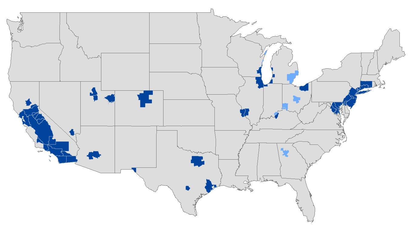
Air Compare
(2012-2021) U.S. Environmental Protection AgencyThis interactive map displays parish-based trends for the five AQI air pollutants that may affect human health. For data limitations specific to this tool, including the pollutants that are accounted for in the analyses, click on the Basic Info tab at the top of the page, then Data Limitations on the right side of the page. Note: For information on the predominant directions in which air pollutants flow, refer to the Wind Rose Plots tool in the Wildfire section.
1. Scroll down until you see the U.S map. 2. In the upper left-hand corner of the map, click on Trends, then select category of interest. 3. Zoom in and click parish of interest to obtain a graph of annual statistics (or hover over the parish for a quick view). Parishes/counties shaded darker blue have data available. You can click multiple parishes to compare locations. Each graph appears above the map. 4. For data broken down into months, click on Seasons in upper left-hand corner, then select group of interest.
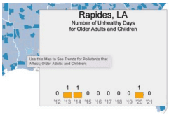
Ozone Exceedances
(1980-present) U.S. Environmental Protection AgencyThis interactive graphing tool compares 8-hour ozone exceedances between two years or multi-year periods for a city or parish. Comparisons are shown by day, month, and year. The ozone exceedance level for this tool is 0.070 ppm.
1. Under Geographic Area, select a City or County (parish) of interest 2. Under Baseline Period, select either a single year or a multi-year average and the range of years in which you are interested. 3. Under Comparison Period, select either a single year or a multi-year average and the range of years in which you are interested in. 4. You may need to uncheck Use ALL Monitors when comparing time periods if data aren’t available for both periods. 5. Click Plot Data.
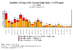
Outdoor Air Quality Data
(Period varies by pollutant; up to 1980- present) U.S. Environmental Protection AgencyThis multi-year tile plotting tool shows the daily AQI pollutant values for a specific location or time period. Each tile represents one day of the year and is color-coded based on the AQI level for that day.
1. Under Pollutant, select pollutant of choice. (e.g., Ozone, All AQI Pollutants) 2. Under Period, select a beginning and ending year (maximum of 25 years). 3. Under Geographical Area, select a city or parish from the drop-down menu. 4. Click Plot Data. The legend is located below the plot.
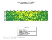
Climate Change Trends
From 2018-2022, 8 of the 17 parishes in Louisiana that record ozone data received a report card grade of C or below for high ozone days from the American Lung Association (2022). Air quality has improved in some areas of Louisiana while other areas, like East Baton Rouge Parish, are still below national standards and struggle with ozone days. Increasing temperatures are tied to increasing ozone levels closer to pollution sources, which cause health issues such as asthma and respiratory problems. A longer wildfire season will also lead to an increased amount of ozone and particulate matter, and a lengthened pollen season will increase the allergens in the air (Nolte et al. 2018). Learn more about future air quality in Climate Change Science and Projection Resources.
Acknowledgements and References
Contributors
- Darrian Bertrand: SCIPP Climate Assessment Specialist, University of Oklahoma
- Rachel Riley: SCIPP Director, University of Oklahoma
- Mark Shafer: SCIPP Deputy Director, University of Oklahoma
Acknowledgements
The original Simple Planning Tool for Louisiana Climate Hazards is a result of SCIPP’s engagement with emergency managers, planners, and other decision makers in Oklahoma, Arkansas, Texas, and Louisiana. We thank the following practitioners for their involvement in various capacities: Robert Hill, Paula Dennison, Danielle O’Neal, Michael McAnelly, and Chance Sparks. We also thank undergraduate student, James Cuellar, and graduate student, Anna Wanless, for their assistance with earlier versions.
A note of thanks is also extended to the individuals who assisted in reviewing sections of and/or provided additional information for the tool, including previous versions: Kristin Calhoun (Cooperative Institute for Mesoscale Meteorological Studies/National Severe Storms Laboratory), Patrick Marsh (NWS Storm Prediction Center), John Nielsen-Gammon (Texas A&M University), Rick Smith (National Weather Service Norman Forecast Office), Vincent Brown (Louisiana State University/Southern Climate Impacts Planning Program), Anna Sitzman (Louisiana State University), and Simone Domingue (University of Oklahoma/Southern Climate Impacts Planning Program).
References
- American Lung Association (ALA), 2022: State of the Air, https://www.lung.org/research/sota.
- American Meteorological Society (AMS), 2020: Glossary of Meteorology, https://glossary.ametsoc.org/wiki/Welcome.
- Bhatia, K., and Coauthors, 2022: A potential explanation for the global increase in tropical cyclone rapid intensification. Nature Communications, 13, 6626 (2022), https://doi.org/10.1038/s41467-022-34321-6.
- Brown, V. M., Keim, B. D., and A. W. Black, 2019: Climatology and trends in hourly precipitation for the southeast United States. Journal of Hydrometeorology, 20(8), 1737-1755, https://journals.ametsoc.org/view/journals/hydr/20/8/jhm-d-19-0004_1.xml.
- Carter, L., A. Terando, K. Dow, K. Hiers, K.E. Kunkel, A. Lascurain, D. Marcy, M. Osland, and P. Schramm, 2018: Southeast. In Impacts, Risks, and Adaptation in the United States: Fourth National Climate Assessment, Volume II [Reidmiller, D.R., C.W. Avery, D.R. Easterling, K.E. Kunkel, K.L.M. Lewis, T.K. Maycock, and B.C. Stewart (eds.)]. U.S. Global Change Research Program, Washington, DC, USA, pp. 743–808. doi: 10.7930/NCA4.2018.CH19.
- Changnon, S.A. and T.R. Karl, 2003: Temporal and spatial variations of freezing rain in the contiguous United States: 1948-2000. J. Appl. Meteor. Climatol., 42, 1302- 1315, https://doi.org/10.1175/1520-0450(2003)042<1302:TASVOF>2.0.CO;2.
- Coastal Protection and Restoration Authority of Louisiana (CPRA), 2023: Louisiana’s Comprehensive Master Plan for a Sustainable Coast. Accessed 1 May 2024, https://coastal.la.gov/wp-content/uploads/2023/06/230531_CPRA_MP_Final-for-web_spreads.pdf.
- Couvillion, B.R., H. Beck, D. Schoolmaster, and M. Fischer, 2017: Land area change in coastal Louisiana 1932 to 2016. U.S. Geological Survey Scientific Investigations Map 3381, 16 pp, https://doi.org/10.3133/sim3381.
- De La Garza, A., 2021: U.S. Civil Engineers Bent the Rules to Give New Orleans Extra Protection from Hurricanes. Those Adjustments Might Have Saved the City During Ida. Time, https://time.com/6094221/hurricane-ida-engineering-protection/.
- Dietz, M. E., K. Liu, and T. A. Bianchette, 2018: Hurricanes as a major driver of coastal erosion in the Mississippi River Delta: A multi-decadal analysis of shoreline retreat rates at Bay Champagne, Louisisna (USA). Water, 10, https://doi.org/10.3390/w10101480.
- Easterling, D.R., K.E. Kunkel, J.R. Arnold, T. Knutson, A.N. LeGrande, L.R. Leung, R.S. Vose, D.E. Wal-iser, and M.F. Wehner, 2017: Precipitation change in the United States. In: Climate Science Special Report: Fourth National Climate Assessment, Volume I [Wuebbles, D.J., D.W. Fahey, K.A. Hibbard, D.J. Dokken, B.C. Stewart, and T.K. Maycock (eds.)]. U.S. Global Change Research Program, Washington, DC, USA, 207-230, doi: 10.7930/J0H993CC.
- Emanuel, K., 2017: Will global warming make hurricane forecasting more difficult? Bulletin of the American Meteorological Society, 98(3), 495-501, https://doi.org/10.1175/BAMS-D-16-0134.1.
- Frankson, R., K. E. Kunkel, S. M. Champion, and J. Nielsen-Gammon, 2022: Louisiana State Climate Summary 2022. NOAA Technical Report NESDIS 150-LA. NOAA/NESDIS, Silver Spring, MD, 6 pp, https://statesummaries.ncics.org/chapter/la/.
- Hayhoe, K., D.J. Wuebbles, D.R. Easterling, D.W. Fahey, S. Doherty, J. Kossin, W. Sweet, R. Vose, and M. Wehner, 2018: Our Changing Climate. In Impacts, Risks, and Adaptation in the United States: Fourth National Climate Assessment, Volume II [Reidmiller, D.R., C.W. Avery, D.R. Easterling, K.E. Kunkel, K.L.M. Lewis, T.K. Maycock, and B.C. Stewart (eds.)]. U.S. Global Change Research Program, Washington, DC, USA, pp. 72–144. doi: 10.7930/NCA4.2018.CH2.
- Himmelstoss, E. A., M. G. Kratzmann, and E. R. Thieler, 2017: National Assessment of Shoreline Change – Summary Statistics for Updated Vector Shorelines and Associated Shoreline Change Data for the Gulf of Mexico and Southeast Atlantic Coasts. U.S. Geological Survey Open-File Report 2017-1015, 8 pp, https://doi.org/10.3133/ofr20171015.
- Kossin, J.P., T. Hall, T. Knutson, K.E. Kunkel, R.J. Trapp, D.E. Waliser, and M.F. Wehner, 2017: Extreme storms. In: Climate Science Special Report: Fourth National Climate Assessment, Volume I [Wuebbles, D.J., D.W. Fahey, K.A. Hibbard, D.J. Dokken, B.C. Stewart, and T.K. Maycock (eds.)]. U.S. Global Change Research Program, Washington, DC, USA, 257-276, doi: 10.7930/J07S7KXX.
- Louisiana Department of Agriculture and Forestry (LDAF), 2022: Protection. https://www.ldaf.state.la.us/forestry/protection/.
- Louisiana Sea Grant, 2024: Ocean Commotion: Fast Facts. Accessed 2 May 2024, https://www.laseagrant.org/education/projects/ocean-commotion/facts/.
- Muis, S., M. Verlaan, H. C. Winsemius, J. Aerts, and P. Ward, 2016: A global reanalysis of storm surges and extreme sea levels. Nature Communications, 7, https://doi.org/10.1038/ncomms11969.
- Mostafiz, R. B., C. J. Friedland, R. V. Rohli, and N. Bushra, 2022: Estimating future residential property risk associated with wildfires in Louisiana, USA. Climate, 10(4), 26 pp, https://doi.org/10.3390/cli10040049.
- National Hurricane Center (NHC), 2022a: Surge Overview. https://www.nhc.noaa.gov/surge/.
- National Hurricane Center (NHC), 2022b: Storm Surge Frequently Asked Questions. https://www.nhc.noaa.gov/surge/faq.php#2.
- National Ocean Service (NOS), 2021: What Is High Tide Flooding? https://oceanservice.noaa.gov/facts/high-tide-flooding.html.
- National Oceanic and Atmospheric Administration (NOAA), 2022: The State of High Tide Flooding and Annual Outlook. https://tidesandcurrents.noaa.gov/HighTideFlooding_AnnualOutlook.html.
- National Weather Service (NWS), 2009: National Weather Service Glossary, w1.weather.gov/glossary.
- National Weather Service (NWS), 2018, personal communication with Rick Smith, National Weather Service Norman Forecast Office.
- National Weather Service (NWS), 2024: Beaufort Wind Scale. Accessed 30 April 2024, https://www.weather.gov/mfl/beaufort.
- Nielsen-Gammon, J. and Coauthors, 2021. Assessment of Historic and Future trends of Extreme Weather in Texas, 1900-2036. Texas A&M University, Office of the Texas State Climatologist, 42 pp, https://climatexas.tamu.edu/files/ClimateReport-1900to2036-2021Update.
- Nolte, C.G., P.D. Dolwick, N. Fann, L.W. Horowitz, V. Naik, R.W. Pinder, T.L. Spero, D.A. Winner, and L.H. Ziska, 2018: Air Quality. In Impacts, Risks, and Adaptation in the United States: Fourth National Climate Assessment, Volume II [Reidmiller, D.R., C.W. Avery, D.R. Easterling, K.E. Kunkel, K.L.M. Lewis, T.K. Maycock, and
- B.C. Stweart (eds.)]. U.S. Global Change Research Prgram, Washington, DC, USA, pp. 512-538. doi: 10.7930/NCA4.2018.CH13.
- Reed, D., Y. Wang, E. Meselhe, and E. White, 2020: Modeling wetland transitions and loss in coastal Louisiana under scenarios of future sea-level rise.
- Geomorphology, 352, https://doi.org/10.1016/j.geomorph.2019.106991.
- Schultz, C.J., W.A. Petersen, and L.D. Carey, 2011: Lightning and severe weather: A comparison between total and cloud-to-ground lightning trends. Weather and Forecasting, 26, 744-755, https://doi.org/10.1175/WAF-D-10-05026.1.
- Sills, G. L., N. D. Vroman, R. E. Wahl, and N. T. Schwanz, 2008: Overview of New Orleans levee failures: Lessons learned and their impact on national levee design and assessment. Journal of Geotechnical and Geoenvironmental Engineering, 134(5), 556-565, https://doi.org/10.1061/(ASCE)1090-0241(2008)134:5(556).
- Stevenson, D. A., and R. P. McCulloh, 2001: Earthquakes in Louisiana. Louisiana Geological Survey Public Information Series No. 7, 8 pp, https://www.lsu.edu/lgs/publications/products/Free_publications/La-earthquakes.pdf.
- Storm Prediction Center (SPC), 2016: 30-year Severe Weather Climatology. https://www.spc.noaa.gov/wcm/#30yrclimo.
- Stein, S., R.J. Geller, M. Liu, 2012: Why earthquake hazard maps often fail and what to do about it, Tectonophysics, 562-563, 1-25, https://doi.org/10.1016/j.tecto.2012.06.047.
- Sweet, W.V., and Coauthors, 2022: Global and Regional Sea Level Rise Scenarios for the United States: Updated Mean Projections and Extreme Water Level Probabilities Along U.S. Coastlines. NOAA Technical Report NOS 01. National Oceanic and Atmospheric Administration, National Ocean Service, Silver Spring, MD, 111 pp., https://oceanservice.noaa.gov/hazards/sealevelrise/sealevelrise-tech-report-sections.html.
- Tracking California, 2021: Air Quality Measures and Limitations. https://trackingcalifornia.org/air-quality/air-contaminant-regulation-and-monitoring.
- University Corporation for Atmospheric Research (UCAR), 2020: What is Air Quality? https://scied.ucar.edu/learning-zone/air-quality/what-is-air-quality#:~:text=Poor%20air%20quality%2C%20which%20contains,air%20at%20a%20particular%20location.
- U.S. Drought Monitor (USDM), 2022: Drought Classification. https://droughtmonitor.unl.edu/About/AbouttheData/DroughtClassification.aspx.
- U.S. Federal Government, 2021: Coastal Erosion. U.S. Climate Resilience Toolkit, Accessed 29 April 2024, https://toolkit.climate.gov/topics/coastal-flood-risk/coastal-erosion.
- U.S. Geological Survey (USGS), 2018: Earthquake Glossary. earthquake.usgs.gov/learn/glossary/?term=earthquake.
- U.S. Geological Survey (USGS), 2019: Saltwater Intrusion. https://www.usgs.gov/mission-areas/water-resources/science/saltwater-intrusion?qt- science_center_objects=0#qt-science_center_objects.
- U.S. Global Change Research Program (USGCRP), 2019: Coastal Erosion. U.S. Climate Resilience Toolkit, https://toolkit.climate.gov/topics/coastal-flood- risk/coastal-erosion.
- U.S. Society on Dams (USSD), 2018: Glossary. https://www.ussdams.org/resource-center/glossary.
- Vose, R.S., D.R. Easterling, K.E. Kunkel, A.N. LeGrande, and M.F. Wehner, 2017: Temperature changes in the United States. In: Climate Science Special Report: Fourth National Climate Assessment, Volume I [Wuebbles, D.J., D.W. Fahey, K.A. Hibbard, D.J. Dokken, B.C. Stewart, and T.K. Maycock (eds.)]. U.S. Global Change Research Program, Washington, DC, USA, 185-206, doi:10.7930/J0N29V45.
- Walsh, K.J.E., J.L. McBride, P.J. Klotzbach, S. Balachandran, S.J. Camargo, G. Holland, T.R. Knutson, J.P. Kossin, T. Lee, A. Sobel, and M. Sugi, 2015: Tropical Cyclones and Climate Change. WIREs Clim Change, 7, 65-89, doi: 10.1002/wcc.371.
- Wehner, M.F., J.R. Arnold, T. Knutson, K.E. Kunkel, and A.N. LeGrande, 2017: Droughts, floods, and wildfires. In: Climate Science Special Report: Fourth National Climate Assessment, Volume I [Wuebbles, D.J., D.W. Fahey, K.A. Hibbard, D.J. Dokken, B.C. Stewart, and T.K. Maycock (eds.)]. U.S. Global Change Research Program, Washington, DC, USA, 231-256, doi: 10.7930/J0CJ8BNN.
- World Meteorological Organization (WMO), 2016: Guidelines on the Definition and Monitoring of Extreme Weather and Climate Events. https://ane4bf-datap1.s3- eu-west-1.amazonaws.com/wmocms/s3fs- public/event/related_docs/DraftversionoftheGuidelinesontheDefinitionandMonitoringofExtremeWeatherandClimateEvents.pdf?h2Kr0f7dXp6CXZzoclQYv eoEQ9FNoO5r.
- Wuebbles, D.J., D.R. Easterling, K. Hayhoe, T. Knutson, R.E. Kopp, J.P. Kossin, K.E. Kunkel, A.N. LeGrande, C. Mears, W.V. Sweet, P.C. Taylor, R.S. Vose, and M.F. Wehner, 2017a: Our globally changing climate. In: Climate Science Special Report: Fourth National Climate Assessment, Volume I [Wuebbles, D.J., D.W. Fahey, K.A. Hibbard, D.J. Dokken, B.C. Stewart, and T.K. Maycock (eds.)]. U.S. Global Change Research Program, Washington, DC, USA, 35-72, doi: 10.7930/J08S4N35.
- Wuebbles, D.J., D.W. Fahey, K.A. Hibbard, B. DeAngelo, S. Doherty, K. Hayhoe, R. Horton, J.P. Kossin, P.C. Taylor, A.M. Waple, and C.P. Weaver, 2017b: Executive Summary of the Climate Science Special Report: Fourth National Climate Assessment, Volume I [Wuebbles, D.J., D.W. Fahey, K.A. Hibbard, D.J. Dokken, B.C. Stewart, and T.K. Maycock (eds.)]. U.S. Global Change Research Program, Washington, DC, USA, 12-34, doi: 10.7930/J0DJ5CTG.
Historical FEMA/Presidential Disaster Declarations by State, Parish, or Tribal Nation
The data visualization interactive reference page below displays statistics of disaster declarations for both states and tribal nations, dating back to 1953.
Disaster Declarations for States and Counties
This page contains an interactive tool that allows the exploration of historic federal disaster declarations by state, parish, hazard, and year. To access information from this page, first select a date range and state/territory from the menus. Information on federally declared disasters within the selected region will be displayed below.
The tool provides the following information:
- Number of disasters by hazard type, county, year, and month,
- The cumulative number of disasters by hazard type, and
- The complete list of federal disaster declarations.
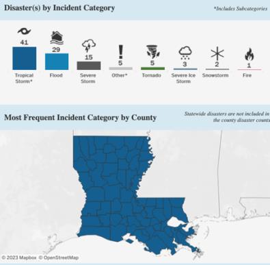
Disaster Declarations for Tribal Nations
This page contains an interactive tool that allows the exploration of historic federal disaster declarations by tribal nation, hazard, and year. To access information from this page, first select a tribal nation from the drop-down list. Information on federally declared disasters within the selected region will be displayed below, organized by natural hazard. The in-depth analysis of a selected tribal nation will be similar to the information provided for disaster declarations of states and counties/parishes above.
Note: Not all of Louisiana’s Tribal Nations are currently represented in this tool because they 1) have not yet declared a disaster, 2) have not met FEMA’s financial threshold, or 3) have received assistance through the state instead of directly from FEMA. The amended 2013 Stafford Act allowing federally recognized tribes to directly declare disasters required a minimum threshold of $1 million in damages. This large amount made it difficult for tribes to independently qualify for declarations. Beginning in January 2017, however, FEMA released pilot guidance which reduces the disaster declaration eligibility threshold to $250,000. More information on this pilot guidance can be accessed here: https://www.fema.gov/disaster/tribal-declarations.

Climate Change Science and Projection Resources
The Louisiana page of the Simple Planning Tool for Climate Hazards is geared towards providing Louisianans with the most accurate and trustworthy data sources. The tool also identifies future climate trends for each hazard. As mentioned in the A Note About Climate Change section (under Instructions and Notes), below is a list of credible, up-to-date climate change science resources to consider for additional information beyond what the Simple Planning Tool provides.
Louisiana State Climate Summary
(2022)NOAA National Centers for Environmental InformationThis report from the NOAA National Centers for Environmental Information (NCEI) provides a state-specific summary of observed and projected changes in Louisiana’s climate, including the change in extreme weather events that affect the state. Three key messages of the summary highlights are provided at the beginning of the report. The NOAA State Climate Summaries were originally created to put National Climate Assessment information into a state-level context.

The 5th National Climate Assessment
(2023)U.S. Global Change Research ProgramNational Climate Assessments synthesize scientific information and evaluate the state of the science on climate change to inform a broad audience of decision-makers across the country. The NCA is mandated by the Global Change Research Act of 1990 and is produced approximately every years. The 5th National Climate Assessment (NCA5) was released in November 2023 and builds upon the work of the four previous assessments. This report was produced by the U.S. Global Change Research Program, which comprises 14 Federal member agencies. NCA5 was written by a diverse team of more than 500 authors and went through multiple rounds of extensive agency review, public comment, and an external peer review conducted by the National Academies of Sciences, Engineering, and Medicine.
NCA5 is a technical scientific assessment of climate change-related risks, impacts, and responses in the United States. The assessment includes 32 chapters on physical science, national-level sectors (e.g., water, energy, agriculture, infrastructure, etc.), regional impacts, and responses (mitigation and adaptation). The regional chapter for Louisiana is Chapter 22: Southeast, but you can find relevant information throughout the report.
Sea Level Rise Technical Report
(2022)This multi-agency report is a product of the Sea Level Rise and Coastal Flood Hazard and Tools Interagency Task Force and provides the most up-to-date sea level rise projections through 2150 for all U.S. coastal waters. This report synthesizes the science of sea level rise, informs decision makers and communities about their potential risks from current and future sea level rise, and is a key input to the Fifth National Climate Assessment (NCA5). A Companion Application Guide to integrate this information into planning processes and adaptation decisions is accessible at https://oceanservice.noaa.gov/hazards/sealevelrise/sealevelrise-tech-report-sections.html#application-guide (click Download the Companion Application Guide to access the document).
Climate of the Gulf Coast States: An Examination of Climate Change’s Effects Across the Region
(2021)This four-chapter report is a product of FloodWise Communities, a National Academy of Sciences Gulf Research Program project led by the Southern Climate Impacts Planning Program (SCIPP), the Great Lakes Integrated Sciences and Assessments (GLISA), and the University of Oklahoma. The document includes an in-depth examination of the climate in TX, LA, AL, MS, GA, and FL. The chapters include: Geography and Average Climatology, Observed Changes in the Climate, Climate Modeling and Future Climate Change, and Climate Hazards.
NCA4 Volume I: Climate Science Special Report
(2017)U.S. Global Change Research ProgramThis stand-alone report is an authoritative assessment of the science relating to climate change and its physical impacts, with a focus on the U.S. Released in November 2017, it was led by NOAA, represents the first of two volumes of the NCA4, and is mandated by the Global Change Research Act of 1990. The CSSR is designed to serve as the foundation for efforts to assess climate-related risks and inform decision-making about responses. The report provides 1) an updated detailed analysis of the findings of how climate change is affecting weather and climate across the United States; 2) an executive summary and other materials that provides the basis for the discussion of climate science found in the second volume of the NCA4; and 3) foundational information and projections for climate change, including extremes, to improve “end-to- end” consistency in sectoral, regional, and resilience analyses.
Attribution of Extreme Weather Events in the Context of Climate Change
(2016)(To access for free, the report can be viewed online or a PDF can be downloaded by creating a free account.)
This National Academies of Sciences, Engineering, and Medicine report examines the current state of science of extreme weather attribution and identifies ways to move the science forward to improve attributing capabilities. The following infographic provides an overview of the report and how climate change is affecting extreme weather: https://www.nap.edu/resource/21852/extremeweather-infographic.pdf.
Incentive and Action Programs for Hazard Risk Reduction
Below is a list of resources providing information on incentive and action programs intended to assist in reducing hazard risk for your community. The list is not comprehensive. Please reference the provided links for more information on each program.
All Hazards
Integrating Hazards into the Comprehensive Plan – Webinar (https://www.planningforhazards.com/webinars, scroll to bottom of page): This one-hour webinar focuses on how local governments and communities can reduce their risk and vulnerability by integrating hazard risk reduction strategies into their comprehensive plan. Colorado planners describe the processes, practices used, and lessons they learned when integrating hazards into their comprehensive plans. This webinar was developed in consideration for Colorado, but concepts can be similarly applied and adapted for Louisiana.
Louisiana Mitigation Assistance Resource Guide (https://www.fema.gov/sites/default/files/documents/fema_mitigation-assistance-resource-guide-louisiana.pdf): FEMA Region 6 created this guide to compile many federal and state resources that offer potential funding or technical assistance for mitigation projects into one place. The guide includes a table with the program/resource name, resource type (grant, loan, or technical assistance), hazards addressed, and mitigation type (education and outreach, natural systems protection, planning and regulations, or structure and infrastructure). It also provides more details about the resource and next steps for Louisiana communities.
Natural Hazard Mitigation Saves: 2019 Report (https://www.nibs.org/projects/natural-hazard-mitigation-saves-2019-report): The National Institute of Building Sciences issued this report to highlight the benefit of four broad avenues for implementing mitigation strategies. (1) The Institute’s project team analyzed 23 years of federally funded mitigation grants and found that hazard mitigation funding can save the nation $6 in future disaster costs for every $1 spent. (2) The team looked at scenarios that focus on designing new buildings to exceed provisions of the 2015 model building codes, and the findings revealed that investing in exceeding these building codes can save the nation $4 for every $1 spent. (3) They analyzed benefits of adopting 2018 I-Codes vs. 1990-era design for buildings and found that there’s a national benefit of $11 for every $1 spent. (4) The team looked at private sector retrofit for older buildings. Utilizing more modern retrofitting on existing residential buildings produces $4 of national benefit for every $1 invested.
Flooding
National Flood Insurance Program (NFIP) (https://www.fema.gov/national-flood-insurance-program): This program “aims to reduce the impact of flooding on private and public structures by providing affordable insurance and encouraging communities to adopt and enforce floodplain management regulations. These efforts help mitigate the effects of flooding on new and improved structures…and reduces the socio-economic impacts of disasters.”
NFIP Community Rating System (CRS) (https://www.fema.gov/national-flood-insurance-program-community-rating-system#): CRS “is a voluntary incentive program that recognizes and encourages community floodplain management activities that exceed the minimum NFIP requirements.” As a result, community participation reduces policyholder flood insurance rates and ultimately flood damage to insurable property.
Wildfire
Wildfire Risk to Communities (https://wildfirerisk.org/reduce-risk/): This website provides a list of resources and programs for communities to reduce and manage wildfire risk. The available topics include home ignition-resistant homes, land use planning, evacuation and readiness, equitable risk reduction, smoke ready, prevent ignitions, response, hazards fuel management, recovery and rebuilding, and funding. Under any of these topics, users can view relevant information and community tools, including programs available to take action for the community.
Close SectionOther Miscellaneous Resources
Below is a list of resources that did not fit into any of the other sections, but the authors still felt were useful to include:
Plans and Adaptation Strategies
Louisiana Climate Action Plan (https://gov.louisiana.gov/assets/docs/CCI-Task-force/CAP/Climate_Action_Plan_FINAL_3.pdf): Louisiana’s first Climate Action Plan was released in 2022 and “contains 28 strategies and 84 specific actions to reduce GHG [greenhouse gas] emissions across the entire state economy.” It also strives to “improve equity, public health and quality of life, preserve and protect the environment, build confidence and awareness among the public, and make [Louisiana] more resilient and adaptable to changing environmental conditions.”
Louisiana State Hazard Mitigation Plan (https://gohsep.la.gov/media/publications/2019HM-plan-final.pdf): The Louisiana State Hazard Mitigation Plan was most recently updated in 2019 and prepared by the Louisiana Governor’s Office of Homeland Security and Emergency Preparedness. The plan provides an assessment of natural hazards in Louisiana, capabilities to mitigate impacts to the hazards, and mitigation strategies.
Louisiana Coastal Master Plan (https://coastal.la.gov/our-plan/2017-coastal-master-plan/): Louisiana’s Comprehensive Master Plan for a Sustainable Coast was produced in 2017 by the Coastal Protection and Restoration Authority (CPRA) of Louisiana. It builds off previous Coastal Master Plans and focuses on minimizing coastal land loss by modeling proposed restoration and flood protection projects and creating a prioritization structure for projects. The next plan will be released in 2023 with updated information. The Master Plan Data Viewer with 2017 Coastal Master Plan projects and flood risk reduction resources can be found on the CPRA’s Spatial Viewer Portal (https://cims.coastal.la.gov/MapHome.aspx).
Louisiana’s Strategic Adaptations for Future Environments (https://lasafe.la.gov/): The Louisiana Office of Community Development and the Foundation for Louisiana led LA SAFE, which is a multidisciplinary adaptation strategy for coastal Louisiana with adaptation and resilience goals and actions for the next 50 years. This site includes the Regional Adaptation Strategy and Parish Adaptation Strategy for six coastal parishes that were awarded ~$41 million in Community Development Block Grant funding for flood resilience projects. The LA SAFE mission is “working together for community resilience, economic prosperity, and a better quality of life for everyone in Louisiana.”
Climate Change Adaptation Manual for Louisiana (https://indd.adobe.com/view/31a5da96-9fa2-4a77-8cab-67527094a2b7): The Center for Planning Excellence created this document in 2019 to provide “current and future risks Louisiana’s communities face, and provides policy and program recommendations for elected officials and policy makers, local governments, and residents to reduce current and future risks and build the resilience needed to keep Louisiana’s communities viable and vibrant.” The document also includes adaptation action recommendations, adaptation tools to implement action, and other relevant resources.
Close SectionSPT Feedback
We appreciate your feedback. Please use the Feedback Form for the following:
- Suggest additional tools/resources that SCIPP can consider adding to the SPT. The SCIPP team thoroughly reviews all tools/resources included in the SPT and selects those that are most useful for a range of applications. However, there are tools that we may not be aware of that suit your needs. We’re happy to review other tools and determine if they are a good fit for the SPT. Please provide your contact information in the form if you would like us to respond to you individually.
- Provide comments (negative or positive) or suggestions regarding the SPT.
- Let us know if the SPT has helped you with a plan, risk assessment, etc. We love knowing how the SPT has been valuable!
- Ask for additional advice on the use of a hazard data tool.
You may leave an anonymous comment/suggestion or provide contact information in case there is a need to follow up (optional).
Close Section